Operating SystemsOperating Systems
How a computer manages processes, memory, and files — with the classic exam problems fully worked out.Computer কীভাবে process, memory আর file manage করে — সব classic exam problem step-by-step solve করা আছে।
1. Processes and Threads1. Processes and Threads
An Operating System (OS) is the software that sits between your programs and the hardware. It does four big jobs: it manages the CPU (decides who runs), manages memory (decides who gets RAM), manages files and devices, and gives programs a safe way to talk to hardware through system calls.
A program is a passive file on disk (like a.out). A process is a program that is running. One program can create many processes. A process has: code (text section), data section (global variables), heap (dynamic memory), stack (function calls, local variables), and the current CPU register values.
Operating System (OS) হলো সেই software যা আপনার program আর hardware-এর মাঝখানে থাকে। এর চারটা বড় কাজ: CPU manage করা (কে চলবে ঠিক করা), memory manage করা (কে RAM পাবে), file আর device manage করা, আর system call-এর মাধ্যমে program-কে hardware-এর সাথে নিরাপদে কথা বলার সুযোগ দেওয়া।
Program হলো disk-এ রাখা একটা passive file (যেমন a.out)। Process হলো চলমান (running) program। একটা program থেকে অনেকগুলো process তৈরি হতে পারে। একটা process-এর থাকে: code (text section), data section (global variable), heap (dynamic memory), stack (function call, local variable), আর CPU register-এর বর্তমান মান।
Process Control Block (PCB)Process Control Block (PCB)
The OS keeps one PCB for each process. It is like the ID card + notebook of the process. It stores:
- Process state — new, ready, running, waiting, or terminated.
- Process ID (PID) — a unique number.
- Program counter — address of the next instruction to run.
- CPU registers — saved values of all registers.
- CPU scheduling info — priority, pointers to scheduling queues.
- Memory info — base/limit registers, page tables.
- Accounting info — CPU time used, time limits.
- I/O status — open files, devices in use.
OS প্রতিটা process-এর জন্য একটা করে PCB রাখে। এটা process-এর ID card + notebook-এর মতো। এতে থাকে:
- Process state — new, ready, running, waiting, বা terminated।
- Process ID (PID) — একটা unique number।
- Program counter — পরের instruction-এর address।
- CPU registers — সব register-এর save করা মান।
- CPU scheduling info — priority, scheduling queue-এর pointer।
- Memory info — base/limit register, page table।
- Accounting info — কত CPU time ব্যবহার হয়েছে, time limit।
- I/O status — খোলা file, ব্যবহার করা device।
Process StatesProcess States
A process moves through five states:
- New — the process is being created.
- Ready — it is loaded and waiting for the CPU.
- Running — instructions are executing on the CPU.
- Waiting (Blocked) — it is waiting for an event, like I/O to finish.
- Terminated — it has finished.
একটা process পাঁচটা state-এর মধ্য দিয়ে যায়:
- New — process তৈরি হচ্ছে।
- Ready — load হয়ে গেছে, CPU-এর জন্য অপেক্ষা করছে।
- Running — CPU-তে instruction চলছে।
- Waiting (Blocked) — কোনো event-এর জন্য অপেক্ষা করছে, যেমন I/O শেষ হওয়া।
- Terminated — কাজ শেষ।
Context SwitchContext Switch
When the CPU switches from process A to process B, the OS must save the state of A into A's PCB and load the state of B from B's PCB. This is a context switch. During the switch the CPU does no useful work, so it is pure overhead. Typical time: a few microseconds. More context switches = more wasted time.
CPU যখন process A থেকে process B-তে switch করে, তখন OS-কে A-এর state A-এর PCB-তে save করতে হয় আর B-এর state B-এর PCB থেকে load করতে হয়। এটাই context switch। Switch-এর সময় CPU কোনো কাজের কাজ করে না, তাই এটা পুরোটাই overhead। সাধারণত কয়েক microsecond লাগে। যত বেশি context switch, তত বেশি সময় নষ্ট।
Process vs ThreadProcess vs Thread
A thread is a lightweight unit of execution inside a process. Threads of the same process share the code, data, heap, and open files — but each thread has its own stack, program counter, and registers. Example: in a browser, one thread draws the page while another downloads images.
Thread হলো process-এর ভেতরের একটা lightweight execution unit। একই process-এর thread-গুলো code, data, heap আর open file share করে — কিন্তু প্রতিটা thread-এর নিজস্ব stack, program counter আর register থাকে। উদাহরণ: browser-এ একটা thread page আঁকে, আরেকটা image download করে।
| Pointবিষয় | Process | Thread |
|---|---|---|
| WeightWeight | HeavyweightHeavyweight | LightweightLightweight |
| MemoryMemory | Own address spaceনিজস্ব address space | Shares address space of the processProcess-এর address space share করে |
| Creation costCreation cost | Slow, expensiveধীর, ব্যয়বহুল | Fast, cheapদ্রুত, সস্তা |
| Context switch | Slow (memory map changes)ধীর (memory map বদলায়) | Fast (same address space)দ্রুত (একই address space) |
| Communication | Needs IPC (pipe, shared memory, message)IPC লাগে (pipe, shared memory, message) | Just read/write shared variablesShared variable পড়া/লেখা যথেষ্ট |
| If one crashesএকটা crash করলে | Others surviveবাকিরা বেঁচে থাকে | Whole process may dieপুরো process মরে যেতে পারে |
| Own itemsনিজস্ব জিনিস | Everything (code, data, heap, stack, files)সব কিছু (code, data, heap, stack, files) | Only stack, registers, program counterশুধু stack, register, program counter |
User Threads vs Kernel ThreadsUser Threads vs Kernel Threads
- User-level threads: managed by a library in user space. The kernel does not know about them. Creation and switching are very fast. Problem: if one thread makes a blocking system call, the whole process blocks.
- Kernel-level threads: managed by the OS itself. Slower to create, but the kernel can schedule them on different CPU cores, and one blocked thread does not block the others.
- Mapping models: many-to-one (many user threads on one kernel thread), one-to-one (Linux, Windows), many-to-many.
- User-level thread: user space-এর একটা library manage করে। Kernel এদের কথা জানেই না। তৈরি আর switch খুব দ্রুত। সমস্যা: একটা thread blocking system call দিলে পুরো process block হয়ে যায়।
- Kernel-level thread: OS নিজে manage করে। তৈরি করা ধীর, কিন্তু kernel এদের আলাদা আলাদা CPU core-এ চালাতে পারে, আর একটা block হলে বাকিরা চলতে পারে।
- Mapping model: many-to-one (অনেক user thread এক kernel thread-এ), one-to-one (Linux, Windows), many-to-many।
Multiprogramming vs Multitasking vs Multithreading (Real Exam!)Multiprogramming vs Multitasking vs Multithreading (Real Exam!)
These three words sound alike, but they mean different things. BUET asked to define and compare them (April 2017), so learn them as a set:
- Multiprogramming: keep several jobs in memory at the same time. When the running job blocks (for example, it waits for I/O), the CPU switches to another job. The goal is throughput — the CPU is never idle. The switch happens only when a job blocks, not on a timer.
- Multitasking (time-sharing): the CPU switches between tasks very fast using a timer (preemption), so every user or program feels the machine responds instantly. The goal is responsiveness. It is multiprogramming plus rapid preemptive switching.
- Multithreading: many threads inside ONE process. All threads share the same address space (code, data, heap) but keep their own stack and registers. The goal is parallel work inside one program with cheap creation and cheap switching.
এই তিনটা শব্দ শুনতে একই রকম, কিন্তু মানে আলাদা। BUET এদের define আর compare করতে বলেছিল (April 2017), তাই একসাথে শিখে রাখুন:
- Multiprogramming: একসাথে কয়েকটা job memory-তে রাখা হয়। চলমান job block হলে (যেমন I/O-এর অপেক্ষায়), CPU অন্য job-এ চলে যায়। লক্ষ্য throughput — CPU কখনো বসে থাকে না। Switch হয় শুধু job block হলে, timer-এ নয়।
- Multitasking (time-sharing): CPU একটা timer দিয়ে খুব দ্রুত task বদলায় (preemption), ফলে প্রতিটা user বা program মনে করে machine সাথে সাথে সাড়া দিচ্ছে। লক্ষ্য responsiveness। এটা আসলে multiprogramming + দ্রুত preemptive switching।
- Multithreading: একটা process-এর ভেতরে অনেক thread। সব thread একই address space (code, data, heap) share করে, কিন্তু নিজের stack আর register আলাদা রাখে। লক্ষ্য এক program-এর ভেতরে parallel কাজ — তৈরি আর switch দুটোই সস্তা।
| Pointবিষয় | Multiprogramming | Multitasking | Multithreading |
|---|---|---|---|
| Unit of workকাজের unit | Whole jobs (processes) in memoryMemory-তে পুরো job (process) | Tasks/processes of one or many usersএক বা অনেক user-এর task/process | Threads inside ONE processএকটা process-এর ভেতরের thread |
| Main goalমূল লক্ষ্য | Throughput (keep CPU busy)Throughput (CPU ব্যস্ত রাখা) | Responsiveness (fast feel)Responsiveness (দ্রুত সাড়া) | Parallelism inside one programএক program-এর ভেতরে parallelism |
| Switching triggerSwitch কখন হয় | When the running job blocks (I/O wait)চলমান job block হলে (I/O wait) | Timer interrupt — preemptive time sliceTimer interrupt — preemptive time slice | Scheduler switches threads (cheap, same address space)Scheduler thread বদলায় (সস্তা, একই address space) |
| ExampleExample | Old batch mainframe running jobs back to backপুরনো batch mainframe-এ পরপর job চলা | Your PC running browser + music + editor "at once"আপনার PC-তে browser + গান + editor "একসাথে" চলা | Browser: one thread draws, one downloadsBrowser: এক thread আঁকে, আরেকটা download করে |
fork() — creating a processfork() — process তৈরি করা
In UNIX/Linux, fork() creates a copy of the calling process. The copy is the child. fork() returns 0 to the child and the child's PID to the parent. Both continue running from the line right after fork().
UNIX/Linux-এ fork() calling process-এর একটা copy তৈরি করে। Copy-টা হলো child। fork() child-কে 0 return করে আর parent-কে child-এর PID return করে। দুজনেই fork()-এর পরের লাইন থেকে চলতে থাকে।
#include <stdio.h>
#include <unistd.h>

int main() {
    fork();
    fork();
    printf("Hello\n");
    return 0;
}After the 1st
fork(): 2 processes. After the 2nd fork(): each of the 2 forks again → 4 processes. Each prints once → "Hello" prints 4 times.
General rule: \( n \) fork() calls in a row create \( 2^n \) processes, so the line prints \( 2^n \) times. Number of new child processes created = \( 2^n - 1 \).
১ম
fork()-এর পর: 2টা process। ২য় fork()-এর পর: 2টার প্রত্যেকে আবার fork করে → 4টা process। প্রত্যেকে একবার print করে → "Hello" 4 বার print হয়।
General rule: পরপর \( n \)টা fork() call দিলে \( 2^n \)টা process হয়, তাই লাইনটা \( 2^n \) বার print হয়। নতুন child process-এর সংখ্যা = \( 2^n - 1 \)।
fork() inside an if or a loop. Draw the process tree on paper. Remember: fork() returns 0 in the child, >0 in the parent, and -1 on failure.fork() কোনো if বা loop-এর ভেতরে থাকে। খাতায় process tree এঁকে ফেলুন। মনে রাখুন: fork() child-এ 0, parent-এ >0, আর fail করলে -1 return করে।2. CPU Scheduling2. CPU Scheduling
Many processes wait in the ready queue, but the CPU can run only one at a time (per core). The CPU scheduler picks which process runs next. The goal is to keep the CPU busy and to make users happy.
Scheduling criteria (what we measure):
- CPU utilization — keep the CPU as busy as possible (maximize).
- Throughput — number of processes finished per unit time (maximize).
- Turnaround time — finish time − arrival time. Total time a process spends in the system (minimize).
- Waiting time — total time spent waiting in the ready queue = turnaround time − burst time (minimize).
- Response time — time from arrival until the first time the process gets the CPU (minimize).
Preemptive vs non-preemptive: In non-preemptive scheduling, once a process gets the CPU it keeps it until it finishes or blocks. In preemptive scheduling, the OS can take the CPU away (for example, when the time slice ends or a shorter job arrives).
Ready queue-তে অনেক process অপেক্ষা করে, কিন্তু CPU একসাথে (প্রতি core-এ) একটাই চালাতে পারে। CPU scheduler ঠিক করে পরে কোনটা চলবে। লক্ষ্য: CPU-কে ব্যস্ত রাখা আর user-দের খুশি রাখা।
Scheduling criteria (আমরা কী মাপি):
- CPU utilization — CPU-কে যতটা সম্ভব ব্যস্ত রাখা (maximize)।
- Throughput — প্রতি unit time-এ কয়টা process শেষ হলো (maximize)।
- Turnaround time — finish time − arrival time। System-এ থাকা মোট সময় (minimize)।
- Waiting time — ready queue-তে অপেক্ষার মোট সময় = turnaround time − burst time (minimize)।
- Response time — আসার পর থেকে প্রথমবার CPU পাওয়া পর্যন্ত সময় (minimize)।
Preemptive vs non-preemptive: Non-preemptive scheduling-এ process একবার CPU পেলে শেষ না হওয়া বা block না হওয়া পর্যন্ত রাখে। Preemptive scheduling-এ OS মাঝপথে CPU কেড়ে নিতে পারে (যেমন time slice শেষ হলে বা ছোট job এলে)।
FCFS — First Come, First Served (non-preemptive)FCFS — First Come, First Served (non-preemptive)
Whoever arrives first runs first, like a queue at a shop. Simple, but a long job at the front makes everyone wait.
যে আগে আসে সে আগে চলে, দোকানের লাইনের মতো। সহজ, কিন্তু সামনে একটা লম্বা job থাকলে সবাইকে অপেক্ষা করতে হয়।
| Process | Burst |
|---|---|
| P1 | 24 |
| P2 | 3 |
| P3 | 3 |
Gantt chart:
| P1 | P2 | P3 |
| 0 → 24 | 24 → 27 | 27 → 30 |
| Process | Finish | Turnaround | Waiting |
|---|---|---|---|
| P1 | 24 | 24 − 0 = 24 | 24 − 24 = 0 |
| P2 | 27 | 27 − 0 = 27 | 27 − 3 = 24 |
| P3 | 30 | 30 − 0 = 30 | 30 − 3 = 27 |
Average waiting = (0 + 24 + 27) / 3 = 17. Average turnaround = (24 + 27 + 30) / 3 = 27. If the order were P2, P3, P1, average waiting would be only (0 + 3 + 6)/3 = 3! This is the convoy effect: short processes get stuck behind one long process, like small cars behind a slow truck.
Average waiting = (0 + 24 + 27) / 3 = 17। Average turnaround = (24 + 27 + 30) / 3 = 27। Order যদি P2, P3, P1 হতো, average waiting হতো মাত্র (0 + 3 + 6)/3 = 3! এটাই convoy effect: ছোট process-গুলো একটা লম্বা process-এর পেছনে আটকে যায়, ধীর truck-এর পেছনে ছোট গাড়ির মতো।
SJF — Shortest Job First (non-preemptive)SJF — Shortest Job First (non-preemptive)
Pick the process with the smallest CPU burst. SJF is provably optimal for average waiting time — no other order can beat it. Problem: we usually do not know burst times in advance (we predict them), and long jobs can starve.
সবচেয়ে ছোট CPU burst-এর process-টা বেছে নেয়। Average waiting time-এর জন্য SJF প্রমাণিতভাবে optimal — অন্য কোনো order এর চেয়ে ভালো করতে পারে না। সমস্যা: burst time আগে থেকে জানা যায় না (predict করতে হয়), আর লম্বা job starve করতে পারে।
| Process | Burst |
|---|---|
| P1 | 6 |
| P2 | 8 |
| P3 | 7 |
| P4 | 3 |
Gantt chart (shortest first: P4, P1, P3, P2):
| P4 | P1 | P3 | P2 |
| 0 → 3 | 3 → 9 | 9 → 16 | 16 → 24 |
| Process | Finish | Turnaround | Waiting |
|---|---|---|---|
| P1 | 9 | 9 | 9 − 6 = 3 |
| P2 | 24 | 24 | 24 − 8 = 16 |
| P3 | 16 | 16 | 16 − 7 = 9 |
| P4 | 3 | 3 | 3 − 3 = 0 |
Average waiting = (3 + 16 + 9 + 0) / 4 = 7. Average turnaround = (9 + 24 + 16 + 3) / 4 = 13. FCFS in order P1..P4 would give average waiting 10.25 — SJF wins.
Average waiting = (3 + 16 + 9 + 0) / 4 = 7। Average turnaround = (9 + 24 + 16 + 3) / 4 = 13। P1..P4 order-এ FCFS দিলে average waiting হতো 10.25 — SJF-ই জিতল।
SRTF — Shortest Remaining Time First (preemptive SJF)SRTF — Shortest Remaining Time First (preemptive SJF)
Same idea as SJF, but preemptive: if a new process arrives with a burst shorter than the remaining time of the running process, the new one takes over.
SJF-এর মতোই, কিন্তু preemptive: নতুন কোনো process এলে, তার burst যদি চলমান process-এর remaining time-এর চেয়ে ছোট হয়, তাহলে নতুনটা CPU নিয়ে নেয়।
| Process | Arrival | Burst |
|---|---|---|
| P1 | 0 | 8 |
| P2 | 1 | 4 |
| P3 | 2 | 9 |
| P4 | 3 | 5 |
Step by step:
- t=0: only P1. P1 runs (remaining 8).
- t=1: P2 arrives (burst 4 < P1's remaining 7) → preempt. P2 runs.
- t=2: P3 arrives (9 > P2's remaining 3) → no change.
- t=3: P4 arrives (5 > P2's remaining 2) → no change.
- t=5: P2 finishes. Remaining: P1=7, P3=9, P4=5 → P4 runs.
- t=10: P4 finishes. Remaining: P1=7, P3=9 → P1 runs.
- t=17: P1 finishes → P3 runs until t=26.
Step by step:
- t=0: শুধু P1 আছে। P1 চলে (remaining 8)।
- t=1: P2 আসে (burst 4 < P1-এর remaining 7) → preempt। P2 চলে।
- t=2: P3 আসে (9 > P2-এর remaining 3) → পরিবর্তন নেই।
- t=3: P4 আসে (5 > P2-এর remaining 2) → পরিবর্তন নেই।
- t=5: P2 শেষ। Remaining: P1=7, P3=9, P4=5 → P4 চলে।
- t=10: P4 শেষ। Remaining: P1=7, P3=9 → P1 চলে।
- t=17: P1 শেষ → P3 চলে t=26 পর্যন্ত।
Gantt chart:
| P1 | P2 | P4 | P1 | P3 |
| 0 → 1 | 1 → 5 | 5 → 10 | 10 → 17 | 17 → 26 |
| Process | Finish | Turnaround = Finish − Arrival | Waiting = TAT − Burst |
|---|---|---|---|
| P1 | 17 | 17 − 0 = 17 | 17 − 8 = 9 |
| P2 | 5 | 5 − 1 = 4 | 4 − 4 = 0 |
| P3 | 26 | 26 − 2 = 24 | 24 − 9 = 15 |
| P4 | 10 | 10 − 3 = 7 | 7 − 5 = 2 |
Average waiting = (9 + 0 + 15 + 2) / 4 = 6.5. Average turnaround = (17 + 4 + 24 + 7) / 4 = 13.
Average waiting = (9 + 0 + 15 + 2) / 4 = 6.5। Average turnaround = (17 + 4 + 24 + 7) / 4 = 13।
Priority SchedulingPriority Scheduling
Each process gets a priority number; the highest-priority process runs first (here, smaller number = higher priority). Can be preemptive or non-preemptive. Big problem: starvation — a low-priority process may wait forever. Fix: aging — slowly raise the priority of processes that wait a long time.
প্রতিটা process একটা priority number পায়; সবচেয়ে বেশি priority-র process আগে চলে (এখানে ছোট number = বেশি priority)। Preemptive বা non-preemptive দুটোই হতে পারে। বড় সমস্যা: starvation — কম priority-র process চিরকাল অপেক্ষা করতে পারে। সমাধান: aging — যারা অনেকক্ষণ অপেক্ষা করছে তাদের priority ধীরে ধীরে বাড়ানো।
| Process | Burst | Priority |
|---|---|---|
| P1 | 10 | 3 |
| P2 | 1 | 1 |
| P3 | 2 | 4 |
| P4 | 1 | 5 |
| P5 | 5 | 2 |
Gantt chart (order P2, P5, P1, P3, P4):
| P2 | P5 | P1 | P3 | P4 |
| 0 → 1 | 1 → 6 | 6 → 16 | 16 → 18 | 18 → 19 |
Waiting: P1 = 6, P2 = 0, P3 = 16, P4 = 18, P5 = 1. Average waiting = (6+0+16+18+1)/5 = 8.2.
Waiting: P1 = 6, P2 = 0, P3 = 16, P4 = 18, P5 = 1। Average waiting = (6+0+16+18+1)/5 = 8.2।
Round Robin (RR, preemptive)Round Robin (RR, preemptive)
Every process gets a small fixed time quantum (e.g., 4 ms). If it does not finish in that time, it goes to the back of the ready queue. Great for time-sharing systems: everyone gets a fair turn, response time is good.
প্রতিটা process একটা ছোট নির্দিষ্ট time quantum পায় (যেমন 4 ms)। এর মধ্যে শেষ না হলে সে ready queue-এর পেছনে চলে যায়। Time-sharing system-এর জন্য দারুণ: সবাই fair সুযোগ পায়, response time ভালো।
Gantt chart:
| P1 | P2 | P3 | P1 | P1 | P1 | P1 | P1 |
| 0 → 4 | 4 → 7 | 7 → 10 | 10 → 14 | 14 → 18 | 18 → 22 | 22 → 26 | 26 → 30 |
P2 and P3 finish inside their first quantum (they need only 3). After t=10 only P1 is left, so it runs quantum after quantum.
Waiting: P1 = 30 − 24 = 6 (it waited 4→10), P2 = 4, P3 = 7. Average waiting = (6 + 4 + 7)/3 = 5.67. Average turnaround = (30 + 7 + 10)/3 = 15.67.
P2 আর P3 প্রথম quantum-এর মধ্যেই শেষ (ওদের দরকার মাত্র 3)। t=10-এর পর শুধু P1 বাকি, তাই সে একের পর এক quantum পেয়ে চলে।
Waiting: P1 = 30 − 24 = 6 (সে 4→10 অপেক্ষা করেছে), P2 = 4, P3 = 7। Average waiting = (6 + 4 + 7)/3 = 5.67। Average turnaround = (30 + 7 + 10)/3 = 15.67।
Multilevel QueueMultilevel Queue
The ready queue is split into several queues, e.g., foreground (interactive) using RR and background (batch) using FCFS. Each queue can have its own algorithm, and the queues themselves are scheduled (fixed priority, or time slices like 80% foreground / 20% background). A multilevel feedback queue also lets processes move between queues — a process that uses too much CPU drops to a lower queue; a process that waits too long moves up (this is aging in action).
Ready queue-কে কয়েকটা queue-তে ভাগ করা হয়, যেমন foreground (interactive) চলে RR দিয়ে আর background (batch) চলে FCFS দিয়ে। প্রতিটা queue-র নিজস্ব algorithm থাকতে পারে, আর queue-গুলোর মধ্যেও scheduling হয় (fixed priority, বা 80% foreground / 20% background-এর মতো time ভাগ)। Multilevel feedback queue-তে process queue বদলাতে পারে — বেশি CPU খেলে নিচের queue-তে নামে; বেশি অপেক্ষা করলে উপরে ওঠে (এটাই কার্যত aging)।
| Algorithm | TypeType | Goodভালো দিক | Badখারাপ দিক |
|---|---|---|---|
| FCFS | Non-preemptive | Simple, fair orderসহজ, fair order | Convoy effectConvoy effect |
| SJF | Non-preemptive | Optimal average waitingOptimal average waiting | Needs future knowledge, starvationভবিষ্যৎ জানতে হয়, starvation |
| SRTF | Preemptive | Even better averagesআরও ভালো average | More switches, starvationবেশি switch, starvation |
| Priority | Both possibleদুটোই সম্ভব | Important jobs firstজরুরি কাজ আগে | Starvation (fix: aging)Starvation (সমাধান: aging) |
| Round Robin | Preemptive | Fair, good response timeFair, ভালো response time | Quantum choice is trickyQuantum বাছাই কঠিন |
3. Synchronization3. Synchronization
Race ConditionRace Condition
When two or more processes/threads read and write shared data at the same time, the final result depends on the exact order of execution. This is a race condition.
Concrete example: Two threads both run counter++ once, starting from counter = 5. We expect 7. But counter++ is really three machine steps:
দুই বা ততোধিক process/thread যখন একই সময়ে shared data পড়ে আর লেখে, তখন শেষ ফলাফল নির্ভর করে execution-এর order-এর ওপর। এটাই race condition।
Concrete example: দুইটা thread-ই একবার করে counter++ চালায়, শুরুতে counter = 5। আশা করি ফল হবে 7। কিন্তু counter++ আসলে তিনটা machine step:
register = counter    // read
register = register + 1
counter = register // write- T1: reads counter (5) into its register.
- T2: reads counter (5) into its register. ← T1 has not written yet!
- T1: adds 1 → 6, writes counter = 6.
- T2: adds 1 → 6, writes counter = 6.
- T1: counter (5) নিজের register-এ পড়ে।
- T2: counter (5) নিজের register-এ পড়ে। ← T1 তখনও লেখেনি!
- T1: 1 যোগ করে → 6, counter = 6 লেখে।
- T2: 1 যোগ করে → 6, counter = 6 লেখে।
Critical Section ProblemCritical Section Problem
The critical section is the part of code where a process touches shared data. Only one process should be inside it at a time. A correct solution must satisfy three requirements:
- Mutual exclusion — at most one process in the critical section at any moment.
- Progress — if nobody is inside and someone wants in, the decision cannot be postponed forever; only processes trying to enter take part in the decision.
- Bounded waiting — after a process asks to enter, there is a limit on how many times others can enter before it does (no starvation).
Critical section হলো code-এর সেই অংশ যেখানে process shared data ধরে। একসাথে একটার বেশি process এর ভেতরে থাকা উচিত না। সঠিক সমাধানের তিনটা শর্ত মানতে হয়:
- Mutual exclusion — যেকোনো মুহূর্তে সর্বোচ্চ একটা process critical section-এ।
- Progress — ভেতরে কেউ নেই আর কেউ ঢুকতে চায়, তাহলে সিদ্ধান্ত চিরকাল ঝুলিয়ে রাখা যাবে না; শুধু যারা ঢুকতে চাইছে তারাই সিদ্ধান্তে অংশ নেবে।
- Bounded waiting — কেউ ঢুকতে চাওয়ার পর, তার আগে অন্যরা কতবার ঢুকতে পারবে তার একটা সীমা আছে (starvation নেই)।
Peterson's Solution (two processes)Peterson's Solution (দুই process)
A classic software-only solution for two processes (P0 and P1). It uses two shared variables: flag[2] ("I want to enter") and turn ("it is your turn"). Each process politely gives the turn to the other; whoever's turn it is enters. It satisfies all three requirements (on old simple hardware).
দুই process-এর (P0 আর P1) জন্য classic software-only সমাধান। দুইটা shared variable: flag[2] ("আমি ঢুকতে চাই") আর turn ("তোমার পালা")। প্রতিটা process ভদ্রভাবে অন্যকে পালা দিয়ে দেয়; যার পালা সে ঢোকে। এটা তিনটা শর্তই মানে (পুরনো simple hardware-এ)।
// Process Pi (the other one is Pj)
do {
    flag[i] = true;      // I want to enter
    turn = j;            // but you go first
    while (flag[j] && turn == j)
        ;                // busy wait
    /* critical section */
    flag[i] = false;     // I am out
    /* remainder section */
} while (true);
Mutex LocksMutex Locks
A mutex (mutual exclusion lock) is the simplest tool: acquire() before the critical section, release() after. If the lock is taken, others spin or sleep. A lock where waiting processes keep looping is called a spinlock — it wastes CPU but avoids context switches, so it is good for very short waits on multi-core machines.
Mutex (mutual exclusion lock) হলো সবচেয়ে সহজ tool: critical section-এর আগে acquire(), পরে release()। Lock নেওয়া থাকলে অন্যরা ঘুরতে থাকে বা ঘুমায়। যেখানে অপেক্ষমাণ process loop-এ ঘোরে সেটা spinlock — CPU নষ্ট করে কিন্তু context switch বাঁচায়, তাই multi-core machine-এ খুব ছোট অপেক্ষার জন্য ভালো।
SemaphoresSemaphores
A semaphore S is an integer changed only by two atomic operations:
wait(S)(also called P): decrement S; if S becomes negative, the caller blocks.signal(S)(also called V): increment S; if any process was blocked, wake one up.
Binary semaphore: value only 0 or 1 — works like a mutex. Counting semaphore: value can be any number — counts available copies of a resource (e.g., 5 printers → start S at 5).
Semaphore S একটা integer যা শুধু দুইটা atomic operation দিয়ে বদলায়:
wait(S)(P-ও বলে): S কমায়; S negative হলে caller block হয়।signal(S)(V-ও বলে): S বাড়ায়; কেউ blocked থাকলে একজনকে জাগায়।
Binary semaphore: মান শুধু 0 বা 1 — mutex-এর মতো কাজ করে। Counting semaphore: মান যেকোনো সংখ্যা — resource-এর available copy গোনে (যেমন 5টা printer → S শুরু হয় 5 থেকে)।
Producer–Consumer with SemaphoresProducer–Consumer with Semaphores
A producer puts items into a buffer of size N; a consumer takes them out. We use three semaphores: mutex = 1 (protects the buffer), empty = N (counts empty slots), full = 0 (counts filled slots).
Producer N size-এর একটা buffer-এ item রাখে; consumer সেগুলো নেয়। তিনটা semaphore ব্যবহার হয়: mutex = 1 (buffer পাহারা দেয়), empty = N (খালি slot গোনে), full = 0 (ভরা slot গোনে)।
// Producer                     // Consumer
do {                            do {
    produce item;                   wait(full);
    wait(empty);                    wait(mutex);
    wait(mutex);                    remove item from buffer;
    add item to buffer;             signal(mutex);
    signal(mutex);                  signal(empty);
    signal(full);                   consume item;
} while (true); } while (true);wait(empty) must come before wait(mutex). If you swap them, the producer can hold the mutex and then sleep waiting for an empty slot — the consumer can never get the mutex to make a slot empty → deadlock. MCQs love this trap.wait(empty) অবশ্যই wait(mutex)-এর আগে। উল্টে দিলে producer mutex ধরে রেখে খালি slot-এর অপেক্ষায় ঘুমাতে পারে — consumer আর mutex পাবে না, slot-ও খালি হবে না → deadlock। MCQ-তে এই trap খুব আসে।MonitorsMonitors
Semaphores are easy to misuse (forget a signal, wrong order). A monitor is a high-level language construct: a class where only one process can be active inside at a time, automatically. It also has condition variables with x.wait() (sleep until signaled) and x.signal() (wake one waiting process). Java's synchronized keyword is a monitor idea.
Semaphore ভুলভাবে ব্যবহার করা সহজ (signal ভুলে যাওয়া, ভুল order)। Monitor হলো high-level language construct: এমন একটা class যার ভেতরে একসাথে শুধু একটা process active থাকতে পারে, automatic-ভাবে। এতে condition variable থাকে: x.wait() (signal না পাওয়া পর্যন্ত ঘুম) আর x.signal() (একজন অপেক্ষমাণকে জাগানো)। Java-র synchronized keyword monitor-এরই idea।
4. Deadlocks4. Deadlocks
A deadlock is a situation where a set of processes are all blocked, each waiting for a resource that another process in the set holds. Nobody can move — like two cars facing each other on a one-lane bridge, each waiting for the other to back up.
Deadlock হলো এমন অবস্থা যেখানে একদল process সবাই blocked, প্রত্যেকে এমন resource-এর অপেক্ষায় আছে যা দলের অন্য কেউ ধরে রেখেছে। কেউই নড়তে পারে না — এক লেনের সেতুতে মুখোমুখি দুই গাড়ির মতো, দুজনেই অপেক্ষা করছে অন্যজন পিছাবে বলে।
The 4 Coffman ConditionsThe 4 Coffman Conditions
Deadlock can happen only if all four hold at the same time:
- Mutual exclusion — at least one resource can be used by only one process at a time (e.g., a printer).
- Hold and wait — a process holds one resource while waiting for another.
- No preemption — a resource cannot be taken away by force; the holder must release it voluntarily.
- Circular wait — there is a cycle: P0 waits for P1's resource, P1 waits for P2's, ..., Pn waits for P0's.
Break any one condition and deadlock becomes impossible.
Deadlock তখনই হতে পারে যখন চারটা শর্তই একসাথে সত্য:
- Mutual exclusion — অন্তত একটা resource একসাথে একটা process-ই ব্যবহার করতে পারে (যেমন printer)।
- Hold and wait — একটা process একটা resource ধরে রেখে আরেকটার জন্য অপেক্ষা করে।
- No preemption — জোর করে resource কেড়ে নেওয়া যায় না; ধারককে নিজে ছাড়তে হয়।
- Circular wait — একটা cycle আছে: P0 অপেক্ষা করে P1-এর resource-এর জন্য, P1 করে P2-এর জন্য, ..., Pn করে P0-এর জন্য।
যেকোনো একটা শর্ত ভাঙলেই deadlock অসম্ভব।
Resource Allocation Graph (RAG)Resource Allocation Graph (RAG)
Circles are processes, squares are resources. An edge R → P means "R is assigned to P". An edge P → R means "P is requesting R".
- No cycle → definitely no deadlock.
- Cycle + one instance per resource → definitely deadlock.
- Cycle + multiple instances → deadlock is possible, not certain.
বৃত্ত = process, বর্গ = resource। R → P edge মানে "R এখন P-এর কাছে"। P → R edge মানে "P R চাইছে"।
- Cycle নেই → নিশ্চিতভাবে deadlock নেই।
- Cycle আছে + প্রতি resource-এর একটাই instance → নিশ্চিত deadlock।
- Cycle আছে + একাধিক instance → deadlock হতে পারে, নিশ্চিত না।
Handling StrategiesHandling Strategies
- Prevention — design the system so one Coffman condition can never hold. E.g., order all resources with numbers and always request in increasing order (kills circular wait); request everything at once (kills hold and wait).
- Avoidance — before granting a request, check that the system stays in a safe state (Banker's algorithm). Needs to know maximum needs in advance.
- Detection & recovery — let deadlock happen, run a detection algorithm from time to time, then recover by killing a process or preempting resources.
- Ignore it (Ostrich algorithm) — pretend it never happens. This is what most real OSes (Linux, Windows) actually do, because deadlocks are rare and the other methods are costly.
- Prevention — system এমনভাবে design করা যেন একটা Coffman শর্ত কখনো সত্য না হয়। যেমন: সব resource-কে নম্বর দিয়ে সবসময় বাড়তি order-এ চাওয়া (circular wait শেষ); সব একবারে চাওয়া (hold and wait শেষ)।
- Avoidance — request মঞ্জুর করার আগে দেখা যে system safe state-এ থাকবে কি না (Banker's algorithm)। আগে থেকে maximum need জানতে হয়।
- Detection & recovery — deadlock হতে দাও, মাঝে মাঝে detection algorithm চালাও, তারপর কোনো process মেরে বা resource কেড়ে recover করো।
- Ignore (Ostrich algorithm) — ভান করা যে এমন কিছু হয়ই না। বাস্তবে বেশিরভাগ OS (Linux, Windows) এটাই করে, কারণ deadlock বিরল আর বাকি পদ্ধতিগুলো ব্যয়বহুল।
Banker's Algorithm — full worked example (BUET favorite)Banker's Algorithm — full worked example (BUET favorite)
The system is in a safe state if there exists a safe sequence: an order in which every process can get its maximum need, finish, and return its resources. The algorithm:
- Compute Need = Max − Allocation for each process.
- Set Work = Available.
- Find an unfinished process with Need ≤ Work. Pretend it finishes: Work = Work + its Allocation. Mark it finished.
- Repeat. If all processes can finish → safe. If stuck → unsafe.
System safe state-এ আছে যদি একটা safe sequence থাকে: এমন একটা order যাতে প্রতিটা process তার maximum need পেয়ে, শেষ করে, resource ফেরত দিতে পারে। Algorithm:
- প্রতিটা process-এর জন্য Need = Max − Allocation বের করো।
- Work = Available ধরো।
- এমন একটা অসমাপ্ত process খোঁজো যার Need ≤ Work। ধরো সে শেষ করল: Work = Work + তার Allocation। তাকে finished mark করো।
- Repeat করো। সবাই শেষ করতে পারলে → safe। আটকে গেলে → unsafe।
| Process | Allocation (A B C) | Max (A B C) | Need = Max − Alloc |
|---|---|---|---|
| P0 | 0 1 0 | 7 5 3 | 7 4 3 |
| P1 | 2 0 0 | 3 2 2 | 1 2 2 |
| P2 | 3 0 2 | 9 0 2 | 6 0 0 |
| P3 | 2 1 1 | 2 2 2 | 0 1 1 |
| P4 | 0 0 2 | 4 3 3 | 4 3 1 |
Total allocated = (7, 2, 5), so Available = (10, 5, 7) − (7, 2, 5) = (3, 3, 2). Now run the safety check, Work = (3, 3, 2):
মোট allocated = (7, 2, 5), তাই Available = (10, 5, 7) − (7, 2, 5) = (3, 3, 2)। এবার safety check চালাই, Work = (3, 3, 2):
| Step | Work | CheckCheck | ResultResult | New Work = Work + Alloc |
|---|---|---|---|---|
| 1 | 3 3 2 | P0 needs 7 4 3 ≤ 3 3 2? | No — skipনা — skip | — |
| 2 | 3 3 2 | P1 needs 1 2 2 ≤ 3 3 2? | Yes — P1 runsহ্যাঁ — P1 চলে | 3 3 2 + 2 0 0 = 5 3 2 |
| 3 | 5 3 2 | P2 needs 6 0 0 ≤ 5 3 2? | No — skipনা — skip | — |
| 4 | 5 3 2 | P3 needs 0 1 1 ≤ 5 3 2? | Yes — P3 runsহ্যাঁ — P3 চলে | 5 3 2 + 2 1 1 = 7 4 3 |
| 5 | 7 4 3 | P4 needs 4 3 1 ≤ 7 4 3? | Yes — P4 runsহ্যাঁ — P4 চলে | 7 4 3 + 0 0 2 = 7 4 5 |
| 6 | 7 4 5 | P0 needs 7 4 3 ≤ 7 4 5? | Yes — P0 runsহ্যাঁ — P0 চলে | 7 4 5 + 0 1 0 = 7 5 5 |
| 7 | 7 5 5 | P2 needs 6 0 0 ≤ 7 5 5? | Yes — P2 runsহ্যাঁ — P2 চলে | 7 5 5 + 3 0 2 = 10 5 7 |
All processes can finish. Safe sequence: ⟨P1, P3, P4, P0, P2⟩ → the system is in a safe state. (Other safe sequences also exist, e.g., ⟨P1, P3, P4, P2, P0⟩ — any valid one is a correct answer.)
সব process শেষ করতে পারে। Safe sequence: ⟨P1, P3, P4, P0, P2⟩ → system safe state-এ আছে। (অন্য safe sequence-ও আছে, যেমন ⟨P1, P3, P4, P2, P0⟩ — যেকোনো valid sequence সঠিক উত্তর।)
Handling a new request (Request ≤ Need and Request ≤ Available must both hold): pretend to grant it — Available −= Request, Allocation += Request, Need −= Request — then run the safety check again. If the new state is safe, grant it for real; if not, roll back and make the process wait. Example: P1 requests (1, 0, 2). Check: (1,0,2) ≤ Need(1,2,2) ✓ and ≤ Available(3,3,2) ✓. After pretending: Available = (2,3,0), P1 Alloc = (3,0,2), P1 Need = (0,2,0). The safety check still finds ⟨P1, P3, P4, P0, P2⟩ → grant it.
নতুন request এলে (Request ≤ Need এবং Request ≤ Available দুটোই লাগবে): ধরে নাও দিলাম — Available −= Request, Allocation += Request, Need −= Request — তারপর আবার safety check চালাও। নতুন state safe হলে সত্যিই দাও; না হলে ফিরিয়ে নিয়ে process-কে অপেক্ষা করাও। Example: P1 চায় (1, 0, 2)। Check: (1,0,2) ≤ Need(1,2,2) ✓ এবং ≤ Available(3,3,2) ✓। ধরে নেওয়ার পর: Available = (2,3,0), P1 Alloc = (3,0,2), P1 Need = (0,2,0)। Safety check এখনও ⟨P1, P3, P4, P0, P2⟩ পায় → request মঞ্জুর।
5. Memory Management5. Memory Management
Logical vs Physical Address, MMULogical vs Physical Address, MMU
A logical (virtual) address is what the CPU generates — the address the program sees. A physical address is the real location in RAM. The MMU (Memory Management Unit) is hardware that translates logical → physical at run time. Simplest MMU: a relocation (base) register — physical = logical + base — and a limit register to stop the process from touching others' memory.
Logical (virtual) address হলো CPU যা generate করে — program যে address দেখে। Physical address হলো RAM-এর আসল জায়গা। MMU (Memory Management Unit) হলো hardware যা run time-এ logical → physical translate করে। সবচেয়ে সহজ MMU: relocation (base) register — physical = logical + base — আর limit register যা process-কে অন্যের memory ছুঁতে দেয় না।
Contiguous Allocation: First / Best / Worst FitContiguous Allocation: First / Best / Worst Fit
In contiguous allocation each process gets one continuous block. Free memory has "holes". Where do we put a new process?
- First fit: the first hole that is big enough. Fast.
- Best fit: the smallest hole that is big enough. Leaves tiny useless holes.
- Worst fit: the largest hole. Leaves big leftover pieces.
In practice, first fit and best fit beat worst fit in both speed and memory use.
Contiguous allocation-এ প্রতিটা process একটানা একটা block পায়। Free memory-তে "hole" থাকে। নতুন process কোথায় বসাব?
- First fit: প্রথম যে hole-এ জায়গা হয়। দ্রুত।
- Best fit: জায়গা হয় এমন সবচেয়ে ছোট hole। ছোট ছোট অকেজো hole রেখে যায়।
- Worst fit: সবচেয়ে বড় hole। বড় বড় leftover টুকরা রেখে যায়।
বাস্তবে speed আর memory ব্যবহারে first fit আর best fit — দুটোই worst fit-এর চেয়ে ভালো।
| Process | First fit | Best fit | Worst fit |
|---|---|---|---|
| 212K | 500K hole (288K left)500K hole (288K বাকি) | 300K hole (88K left)300K hole (88K বাকি) | 600K hole (388K left)600K hole (388K বাকি) |
| 417K | 600K hole (183K left)600K hole (183K বাকি) | 500K hole (83K left)500K hole (83K বাকি) | 500K hole (83K left)500K hole (83K বাকি) |
| 112K | 288K hole (176K left)288K hole (176K বাকি) | 200K hole (88K left)200K hole (88K বাকি) | 388K hole (276K left)388K hole (276K বাকি) |
| 426K | must wait (no hole fits)অপেক্ষা করতে হয় (কোনো hole-এ হয় না) | 600K hole (174K left)600K hole (174K বাকি) | must wait (no hole fits)অপেক্ষা করতে হয় (কোনো hole-এ হয় না) |
Here only best fit places all four processes. This exact style of question appears in exams: trace each hole carefully and update leftover sizes.
এখানে শুধু best fit চারটা process-ই বসাতে পারে। Exam-এ ঠিক এই ধাঁচের প্রশ্ন আসে: প্রতিটা hole trace করে leftover size update করতে হয়।
FragmentationFragmentation
- External fragmentation: total free memory is enough, but it is split into small non-contiguous holes, so a big request fails. Happens in contiguous allocation and segmentation. Fix: compaction (shuffle memory together) or use paging.
- Internal fragmentation: memory is given in fixed-size blocks; the unused part inside a block is wasted. Happens in paging (last page is rarely full). Average waste ≈ half a page per process.
- External fragmentation: মোট free memory যথেষ্ট, কিন্তু ছোট ছোট আলাদা hole-এ ভাগ হয়ে আছে, তাই বড় request fail করে। Contiguous allocation আর segmentation-এ হয়। সমাধান: compaction (memory একসাথে ঠেলে আনা) বা paging।
- Internal fragmentation: Memory দেওয়া হয় fixed-size block-এ; block-এর ভেতরের অব্যবহৃত অংশ নষ্ট হয়। Paging-এ হয় (শেষ page প্রায়ই পুরো ভরে না)। গড় অপচয় ≈ process প্রতি আধা page।
PagingPaging
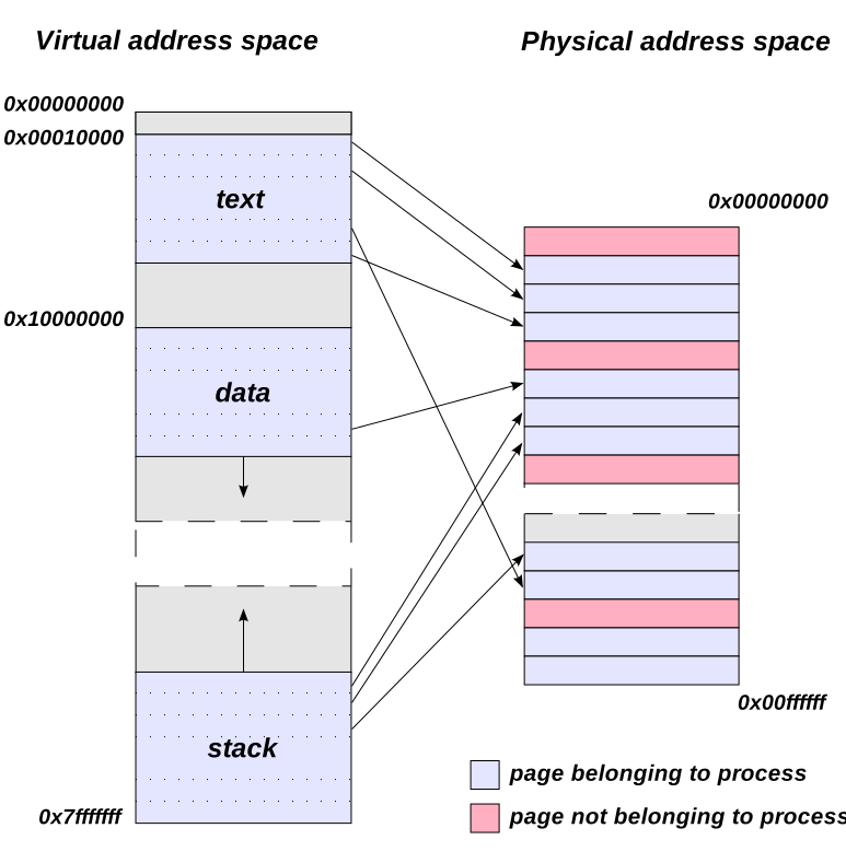
Paging removes external fragmentation. Logical memory is cut into fixed-size pages; physical memory is cut into same-size frames. Any page can go into any free frame — no need to be contiguous. A per-process page table maps page number → frame number.
Address translation: if the page size is \( 2^n \) bytes, the CPU splits a logical address into a page number p (high bits) and an offset d (low n bits):
Paging external fragmentation দূর করে। Logical memory-কে fixed-size page-এ কাটা হয়; physical memory-কে একই size-এর frame-এ। যেকোনো page যেকোনো খালি frame-এ যেতে পারে — একটানা হওয়ার দরকার নেই। প্রতিটা process-এর page table map করে: page number → frame number।
Address translation: page size যদি \( 2^n \) byte হয়, CPU logical address-কে ভাগ করে page number p (উপরের bit) আর offset d (নিচের n bit)-এ:
- Page number p = ⌊3500 / 1024⌋ = 3.
- Offset d = 3500 mod 1024 = 3500 − 3×1024 = 3500 − 3072 = 428.
- Suppose the page table says page 3 → frame 8. Then physical address = 8 × 1024 + 428 = 8620.
- Page number p = ⌊3500 / 1024⌋ = 3।
- Offset d = 3500 mod 1024 = 3500 − 3×1024 = 3500 − 3072 = 428।
- ধরুন page table বলে page 3 → frame 8। তাহলে physical address = 8 × 1024 + 428 = 8620।
- Split the bits: offset needs 12 bits (because \( 4096 = 2^{12} \)). Remaining 16 − 12 = 4 bits for the page number. So there are \( 2^4 = 16 \) pages, each 4096 bytes.
- Logical address = 0x3A7F (= 14975 decimal). In binary:
0011 1010 0111 1111. - Top 4 bits =
0011→ page number p = 3. Low 12 bits =1010 0111 1111= 0xA7F → offset d = 2687. Check: 14975 = 3×4096 + 2687. ✓ - Page table lookup: suppose page 3 → frame 6.
- Physical address = frame × page size + offset = 6 × 4096 + 2687 = 24576 + 2687 = 27263 (= 0x6A7F). Notice the offset bits never change — only the page-number bits are replaced by the frame number.
- Bit ভাগ করুন: offset-এর জন্য 12 bit লাগে (কারণ \( 4096 = 2^{12} \))। বাকি 16 − 12 = 4 bit page number-এর জন্য। তাই page আছে \( 2^4 = 16 \)টা, প্রতিটা 4096 byte।
- Logical address = 0x3A7F (= decimal 14975)। Binary-তে:
0011 1010 0111 1111। - উপরের 4 bit =
0011→ page number p = 3। নিচের 12 bit =1010 0111 1111= 0xA7F → offset d = 2687। Check: 14975 = 3×4096 + 2687। ✓ - Page table lookup: ধরুন page 3 → frame 6।
- Physical address = frame × page size + offset = 6 × 4096 + 2687 = 24576 + 2687 = 27263 (= 0x6A7F)। লক্ষ করুন offset-এর bit কখনো বদলায় না — শুধু page-number-এর bit-গুলোর জায়গায় frame number বসে।
Page Size Trade-offs — small vs large pagesPage Size Trade-offs — ছোট vs বড় page
Advantages of small pages:
- Less internal fragmentation — the wasted space in the last page is on average half a page, so smaller page = less waste. Example: a 13 KB program with 4 KB pages wastes 3 KB in the last page; with 1 KB pages it wastes 0 KB.
- Better fit to locality — memory is loaded in finer pieces, so only the bytes really needed come into RAM. Less useless data is loaded.
Problems of small pages:
- Bigger page table — same address space / smaller page = MORE pages = more page table entries. Example: 32-bit space with 4 KB pages → \( 2^{20} \) entries; with 1 KB pages → \( 2^{22} \) entries (4× bigger table).
- More TLB misses — the TLB has a fixed number of entries; each entry now covers less memory, so its "reach" shrinks and misses go up.
- More page faults and more I/O overhead — bringing the same amount of data needs more separate page transfers, and each disk transfer has a fixed startup cost.
Large pages are the exact mirror: less table/TLB overhead and fewer faults, but more internal fragmentation and more useless data loaded per fault.
ছোট page-এর সুবিধা:
- Internal fragmentation কম — শেষ page-এ গড়ে আধা page নষ্ট হয়, তাই page ছোট হলে অপচয়ও কম। Example: 13 KB program-এ 4 KB page হলে শেষ page-এ 3 KB নষ্ট; 1 KB page হলে 0 KB।
- Locality-র সাথে ভালো মেলে — memory ছোট ছোট টুকরায় load হয়, তাই সত্যিই যা দরকার শুধু সেটাই RAM-এ আসে। অদরকারি data কম load হয়।
ছোট page-এর সমস্যা:
- Page table বড় হয় — একই address space / ছোট page = বেশি page = বেশি page table entry। Example: 32-bit space-এ 4 KB page → \( 2^{20} \) entry; 1 KB page → \( 2^{22} \) entry (4 গুণ বড় table)।
- TLB miss বাড়ে — TLB-র entry সংখ্যা fixed; প্রতিটা entry এখন কম memory cover করে, তাই TLB-র "reach" কমে আর miss বাড়ে।
- Page fault আর I/O overhead বাড়ে — একই পরিমাণ data আনতে বেশি সংখ্যক আলাদা page transfer লাগে, আর প্রতিটা disk transfer-এর একটা fixed startup খরচ আছে।
বড় page ঠিক এর উল্টো: table/TLB overhead কম, fault কম — কিন্তু internal fragmentation বেশি, আর প্রতি fault-এ অদরকারি data বেশি load হয়।
TLB — Translation Lookaside BufferTLB — Translation Lookaside Buffer
The page table lives in RAM, so a plain paged access needs two memory accesses (one for the table, one for the data). The TLB is a small, very fast hardware cache of recent page → frame translations. TLB hit: translation is almost free. TLB miss: go to the page table in memory.
Effective Access Time (EAT): with hit ratio \( h \), memory time \( m \), TLB time \( \epsilon \): \( EAT = h(m + \epsilon) + (1-h)(2m + \epsilon) \). Example: m = 100 ns, ε ≈ 0, h = 0.9 → EAT = 0.9×100 + 0.1×200 = 110 ns.
Page table থাকে RAM-এ, তাই সাধারণ paged access-এ দুইবার memory access লাগে (একবার table, একবার data)। TLB হলো সাম্প্রতিক page → frame translation-এর ছোট, খুব দ্রুত hardware cache। TLB hit: translation প্রায় free। TLB miss: memory-র page table-এ যেতে হয়।
Effective Access Time (EAT): hit ratio \( h \), memory time \( m \), TLB time \( \epsilon \) হলে: \( EAT = h(m + \epsilon) + (1-h)(2m + \epsilon) \)। Example: m = 100 ns, ε ≈ 0, h = 0.9 → EAT = 0.9×100 + 0.1×200 = 110 ns।
SegmentationSegmentation
Segmentation divides a program the way the programmer sees it: code segment, data segment, stack segment, etc. Segments have different sizes. An address is a pair (segment number, offset). The segment table stores each segment's base and limit; the hardware checks offset < limit, then physical = base + offset. Because segments are variable-size, segmentation suffers external fragmentation.
Segmentation program-কে ভাগ করে যেভাবে programmer দেখে: code segment, data segment, stack segment ইত্যাদি। Segment-গুলোর size আলাদা। Address হলো একটা জোড়া (segment number, offset)। Segment table-এ প্রতিটা segment-এর base আর limit থাকে; hardware check করে offset < limit, তারপর physical = base + offset। Segment variable-size বলে segmentation-এ external fragmentation হয়।
| Pointবিষয় | Paging | Segmentation |
|---|---|---|
| Block sizeBlock size | Fixed (page)Fixed (page) | Variable (segment)Variable (segment) |
| Viewদৃষ্টিভঙ্গি | Physical, invisible to programmerPhysical, programmer দেখে না | Logical, matches program structureLogical, program-এর গঠন অনুযায়ী |
| Fragmentation | InternalInternal | ExternalExternal |
| Table storesTable-এ থাকে | Frame numbersFrame number | Base + limitBase + limit |
| Address formAddress-এর রূপ | (page, offset) | (segment, offset) |
6. Virtual Memory6. Virtual Memory
Demand Paging and Page FaultsDemand Paging and Page Faults
Virtual memory lets a program be bigger than RAM. With demand paging, a page is loaded into RAM only when it is first used — "lazy loading". Each page table entry has a valid/invalid bit. Accessing an invalid page triggers a page fault. Steps of a page fault:
- The MMU finds the invalid bit and traps to the OS.
- The OS checks: is this a real invalid access (kill the process) or just a page not yet in RAM?
- Find a free frame (if none, run a page replacement algorithm to evict one; write it to disk if dirty).
- Read the wanted page from disk into the frame.
- Update the page table (valid bit = 1, frame number).
- Restart the instruction that faulted.
Virtual memory-র কারণে program RAM-এর চেয়ে বড় হতে পারে। Demand paging-এ কোনো page প্রথমবার ব্যবহারের সময়ই কেবল RAM-এ আনা হয় — "lazy loading"। প্রতিটা page table entry-তে valid/invalid bit থাকে। Invalid page access করলে page fault হয়। Page fault-এর ধাপ:
- MMU invalid bit পেয়ে OS-কে trap করে।
- OS check করে: এটা কি সত্যিই invalid access (process kill) নাকি page শুধু RAM-এ নেই?
- খালি frame খোঁজে (না থাকলে page replacement algorithm চালিয়ে একটা বের করে; dirty হলে disk-এ লেখে)।
- দরকারি page disk থেকে frame-এ পড়ে।
- Page table update করে (valid bit = 1, frame number)।
- যে instruction-এ fault হয়েছিল সেটা আবার চালায়।
Effective access time with faults: if page fault rate is \( p \), memory access is \( m \), and fault service takes \( F \): \( EAT = (1-p) \times m + p \times F \). Faults are millions of times slower than RAM, so even a tiny \( p \) hurts a lot.
Fault সহ effective access time: page fault rate \( p \), memory access \( m \), fault service time \( F \) হলে: \( EAT = (1-p) \times m + p \times F \)। Fault RAM-এর চেয়ে লাখো গুণ ধীর, তাই খুব ছোট \( p \)-ও অনেক ক্ষতি করে।
Page Replacement — worked examples (BUET favorite)Page Replacement — worked examples (BUET favorite)
We use the classic reference string 7, 0, 1, 2, 0, 3, 0, 4, 2, 3, 0, 3, 2, 1, 2, 0, 1, 7, 0, 1 with 3 frames. In the tables below, each column is one reference; F marks a page fault, H a hit. Frames show their contents after the reference.
Classic reference string 7, 0, 1, 2, 0, 3, 0, 4, 2, 3, 0, 3, 2, 1, 2, 0, 1, 7, 0, 1 আর 3 frame ব্যবহার করব। নিচের table-এ প্রতিটা column একটা reference; F মানে page fault, H মানে hit। Frame-এ reference-এর পরের অবস্থা দেখানো হয়েছে।
FIFO (First-In, First-Out)
Evict the page that has been in memory the longest (the oldest arrival).
যে page সবচেয়ে আগে memory-তে এসেছে (oldest) তাকে বের করে দাও।
| Ref | 7 | 0 | 1 | 2 | 0 | 3 | 0 | 4 | 2 | 3 | 0 | 3 | 2 | 1 | 2 | 0 | 1 | 7 | 0 | 1 |
|---|---|---|---|---|---|---|---|---|---|---|---|---|---|---|---|---|---|---|---|---|
| F1 | 7 | 7 | 7 | 2 | 2 | 2 | 2 | 4 | 4 | 4 | 0 | 0 | 0 | 0 | 0 | 0 | 0 | 7 | 7 | 7 |
| F2 | 0 | 0 | 0 | 0 | 3 | 3 | 3 | 2 | 2 | 2 | 2 | 2 | 1 | 1 | 1 | 1 | 1 | 0 | 0 | |
| F3 | 1 | 1 | 1 | 1 | 0 | 0 | 0 | 3 | 3 | 3 | 3 | 3 | 3 | 2 | 2 | 2 | 2 | 1 | ||
| F/H | F | F | F | F | H | F | F | F | F | F | F | H | H | F | H | F | H | F | F | F |
FIFO: 15 page faults (5 hits).
FIFO: 15 page fault (5 hit)।
Optimal (OPT)
Evict the page that will not be used for the longest time in the future. It gives the minimum possible faults, but it needs future knowledge — so it is only a benchmark to compare against.
যে page ভবিষ্যতে সবচেয়ে দেরিতে ব্যবহার হবে তাকে বের করো। এতে সবচেয়ে কম fault হয়, কিন্তু ভবিষ্যৎ জানতে হয় — তাই এটা শুধু তুলনার benchmark।
| Ref | 7 | 0 | 1 | 2 | 0 | 3 | 0 | 4 | 2 | 3 | 0 | 3 | 2 | 1 | 2 | 0 | 1 | 7 | 0 | 1 |
|---|---|---|---|---|---|---|---|---|---|---|---|---|---|---|---|---|---|---|---|---|
| F1 | 7 | 7 | 7 | 2 | 2 | 2 | 2 | 2 | 2 | 2 | 2 | 2 | 2 | 2 | 2 | 2 | 2 | 7 | 7 | 7 |
| F2 | 0 | 0 | 0 | 0 | 0 | 0 | 0 | 0 | 0 | 0 | 0 | 0 | 0 | 0 | 0 | 0 | 0 | 0 | 0 | |
| F3 | 1 | 1 | 1 | 3 | 3 | 4 | 4 | 3 | 3 | 3 | 3 | 1 | 1 | 1 | 1 | 1 | 1 | 1 | ||
| F/H | F | F | F | F | H | F | H | F | H | F | H | H | H | F | H | H | H | F | H | H |
Optimal: 9 page faults. (At reference 4 we evict 1 because 0 and 2 are needed sooner; at reference 3 we evict 4 because it is never used again.)
Optimal: 9 page fault। (Reference 4-এ 1-কে বের করি কারণ 0 আর 2 আগে লাগবে; reference 3-এ 4-কে বের করি কারণ সে আর কখনো লাগবে না।)
LRU (Least Recently Used)
Evict the page that was not used for the longest time in the past. LRU uses history as a guess of the future. It is close to Optimal and never suffers Belady's anomaly (it is a "stack algorithm").
যে page অতীতে সবচেয়ে দীর্ঘ সময় ব্যবহার হয়নি তাকে বের করো। LRU অতীতকে ভবিষ্যতের অনুমান হিসেবে ব্যবহার করে। এটা Optimal-এর কাছাকাছি আর কখনো Belady's anomaly-তে ভোগে না ("stack algorithm")।
| Ref | 7 | 0 | 1 | 2 | 0 | 3 | 0 | 4 | 2 | 3 | 0 | 3 | 2 | 1 | 2 | 0 | 1 | 7 | 0 | 1 |
|---|---|---|---|---|---|---|---|---|---|---|---|---|---|---|---|---|---|---|---|---|
| F1 | 7 | 7 | 7 | 2 | 2 | 2 | 2 | 4 | 4 | 4 | 0 | 0 | 0 | 1 | 1 | 1 | 1 | 1 | 1 | 1 |
| F2 | 0 | 0 | 0 | 0 | 0 | 0 | 0 | 0 | 3 | 3 | 3 | 3 | 3 | 3 | 0 | 0 | 0 | 0 | 0 | |
| F3 | 1 | 1 | 1 | 3 | 3 | 3 | 2 | 2 | 2 | 2 | 2 | 2 | 2 | 2 | 2 | 7 | 7 | 7 | ||
| F/H | F | F | F | F | H | F | H | F | F | F | F | H | H | F | H | F | H | F | H | H |
LRU: 12 page faults. Summary on this string with 3 frames: Optimal 9 < LRU 12 < FIFO 15.
LRU: 12 page fault। এই string-এ 3 frame-এ সারসংক্ষেপ: Optimal 9 < LRU 12 < FIFO 15।
Belady's AnomalyBelady's Anomaly
Normally more frames → fewer faults. But with FIFO, sometimes more frames give MORE faults. Classic string: 1, 2, 3, 4, 1, 2, 5, 1, 2, 3, 4, 5 — FIFO gives 9 faults with 3 frames but 10 faults with 4 frames. LRU and Optimal never show this anomaly.
সাধারণত frame বাড়লে fault কমে। কিন্তু FIFO-তে কখনো কখনো frame বাড়ালে fault-ও বাড়ে। Classic string: 1, 2, 3, 4, 1, 2, 5, 1, 2, 3, 4, 5 — FIFO-তে 3 frame-এ 9 fault কিন্তু 4 frame-এ 10 fault। LRU আর Optimal-এ এই anomaly কখনো হয় না।
Thrashing and the Working SetThrashing and the Working Set
Thrashing: when a process does not have enough frames, it faults constantly — the system spends more time swapping pages than doing real work. CPU utilization drops, the OS thinks it should add more processes, and things get even worse.
Working set model: the working set is the set of pages a process used in the last \( \Delta \) references (its current "locality"). Give each process at least its working-set size of frames. If the total demand of all processes exceeds the number of frames, suspend some process — that prevents thrashing.
Thrashing: কোনো process যথেষ্ট frame না পেলে সে অনবরত fault করে — system আসল কাজের চেয়ে page swap-এই বেশি সময় দেয়। CPU utilization কমে যায়, OS ভাবে আরও process আনা দরকার, আর অবস্থা আরও খারাপ হয়।
Working set model: শেষ \( \Delta \)টা reference-এ process যে page-গুলো ব্যবহার করেছে সেটাই তার working set (বর্তমান "locality")। প্রতিটা process-কে অন্তত তার working-set size-এর frame দাও। সবার মোট চাহিদা frame সংখ্যার বেশি হলে কোনো process suspend করো — তাতেই thrashing আটকায়।
7. File Systems7. File Systems
Files: Attributes and OperationsFiles: Attributes and Operations
A file is a named collection of related data on storage. Typical attributes: name, identifier (a unique number), type, location on disk, size, protection (who can read/write/execute), timestamps (created/modified/accessed), owner. These attributes are stored in the directory / inode, not inside the file data.
Basic operations: create, open, read, write, seek (reposition), delete, truncate, close. The OS keeps an open-file table with the current position pointer for each open file.
File হলো storage-এ রাখা নামওয়ালা একগুচ্ছ related data। সাধারণ attribute: name, identifier (একটা unique number), type, disk-এ location, size, protection (কে read/write/execute করতে পারবে), timestamp (created/modified/accessed), owner। এই attribute-গুলো থাকে directory / inode-এ, file-এর data-র ভেতরে না।
Basic operation: create, open, read, write, seek (অবস্থান বদলানো), delete, truncate, close। OS একটা open-file table রাখে যাতে প্রতিটা খোলা file-এর current position pointer থাকে।
Directory StructuresDirectory Structures
- Single-level: all files in one directory. Naming clashes, no grouping.
- Two-level: one directory per user. Users are separated, but no sub-grouping.
- Tree: directories inside directories — what Windows/Linux use. Absolute path (from root, e.g.
/home/user/a.txt) vs relative path (from the current directory). - Acyclic graph: a tree plus shared files/directories via links (UNIX hard links, symbolic links). Must be careful about cycles and deletion.
- Single-level: সব file এক directory-তে। নাম নিয়ে সংঘর্ষ, কোনো grouping নেই।
- Two-level: প্রতি user-এর একটা directory। User আলাদা, কিন্তু ভেতরে sub-grouping নেই।
- Tree: Directory-র ভেতরে directory — Windows/Linux এটাই ব্যবহার করে। Absolute path (root থেকে, যেমন
/home/user/a.txt) vs relative path (current directory থেকে)। - Acyclic graph: Tree + link দিয়ে shared file/directory (UNIX hard link, symbolic link)। Cycle আর deletion নিয়ে সাবধান থাকতে হয়।
Allocation MethodsAllocation Methods
How do we place a file's blocks on disk?
- Contiguous: the file occupies consecutive blocks. Directory stores (start, length).
- Linked: each block stores a pointer to the next block. Directory stores (first, last). FAT (File Allocation Table) is a smarter version: all the "next" pointers live in one table in memory.
- Indexed: one index block holds the addresses of all data blocks. Directory points to the index block.
File-এর block-গুলো disk-এ কীভাবে রাখব?
- Contiguous: File পাশাপাশি block-এ থাকে। Directory-তে থাকে (start, length)।
- Linked: প্রতিটা block-এ পরের block-এর pointer থাকে। Directory-তে থাকে (first, last)। FAT (File Allocation Table) এর চালাক version: সব "next" pointer memory-র এক table-এ থাকে।
- Indexed: একটা index block-এ সব data block-এর address থাকে। Directory index block-কে point করে।
| Pointবিষয় | Contiguous | Linked | Indexed |
|---|---|---|---|
| Random (direct) accessRandom (direct) access | Excellentচমৎকার | Very bad (must walk the chain)খুব খারাপ (chain ধরে হাঁটতে হয়) | Good (one index lookup)ভালো (একটা index lookup) |
| External fragmentationExternal fragmentation | Yes — the big problemহ্যাঁ — বড় সমস্যা | Noনেই | Noনেই |
| File growthFile বড় হওয়া | Hard (may need to move the file)কঠিন (file সরাতে হতে পারে) | Easy (add a block anywhere)সহজ (যেকোনো জায়গায় block যোগ) | Easy up to index limitsIndex-এর সীমা পর্যন্ত সহজ |
| OverheadOverhead | None per blockBlock প্রতি নেই | Pointer in every block; bad reliability (one lost pointer breaks the chain)প্রতি block-এ pointer; reliability খারাপ (একটা pointer হারালে chain ভাঙে) | Extra index block per fileFile প্রতি বাড়তি index block |
| Used byব্যবহার করে | CD-ROMs, old systemsCD-ROM, পুরনো system | FAT (MS-DOS) | UNIX inode, ext familyUNIX inode, ext family |
The inode IdeaThe inode Idea
UNIX uses inodes: one inode per file stores the attributes plus a mixed index — typically 12 direct pointers (to data blocks), 1 single indirect (points to a block full of pointers), 1 double indirect, and 1 triple indirect. Small files are fast (direct pointers), and huge files are still possible (indirect levels).
UNIX inode ব্যবহার করে: প্রতি file-এর একটা inode-এ attribute + একটা মিশ্র index থাকে — সাধারণত 12টা direct pointer (data block-এ), 1টা single indirect (pointer-ভরা একটা block-কে point করে), 1টা double indirect, আর 1টা triple indirect। ছোট file দ্রুত (direct pointer), আবার বিশাল file-ও সম্ভব (indirect level)।
- Direct: 12 × 1 KB = 12 KB
- Single indirect: 256 × 1 KB = 256 KB
- Double indirect: 256 × 256 × 1 KB = 64 MB
- Triple indirect: 256 × 256 × 256 × 1 KB = 16 GB
- Direct: 12 × 1 KB = 12 KB
- Single indirect: 256 × 1 KB = 256 KB
- Double indirect: 256 × 256 × 1 KB = 64 MB
- Triple indirect: 256 × 256 × 256 × 1 KB = 16 GB
Free Space ManagementFree Space Management
- Bit map (bit vector): one bit per block — 1 = free, 0 = used (or the opposite). Easy to find n consecutive free blocks; needs extra memory. Example: a 1 TB disk with 4 KB blocks needs 228 bits = 32 MB of bitmap.
- Linked list: free blocks are chained together. No wasted space, but slow to traverse and hard to grab contiguous runs.
- Grouping / counting: store addresses of many free blocks in one block, or store (start, count) pairs for runs of free blocks.
- Bit map (bit vector): প্রতি block-এ এক bit — 1 = free, 0 = used (বা উল্টো)। পরপর n-টা free block খোঁজা সহজ; বাড়তি memory লাগে। Example: 4 KB block-এর 1 TB disk-এ লাগে 228 bit = 32 MB bitmap।
- Linked list: Free block-গুলো chain করা থাকে। জায়গা নষ্ট হয় না, কিন্তু traverse ধীর আর পরপর block পাওয়া কঠিন।
- Grouping / counting: এক block-এ অনেক free block-এর address রাখা, বা free run-এর (start, count) জোড়া রাখা।
Journaling (briefly)Journaling (সংক্ষেপে)
If power fails in the middle of a file operation, the file system can be left half-updated (metadata pointing to garbage). A journaling file system (ext4, NTFS) first writes the planned changes to a journal (log), then applies them, then marks them done. After a crash, the OS replays or discards journal entries — recovery takes seconds instead of a full disk scan (like old fsck).
File operation-এর মাঝখানে power চলে গেলে file system আধা-update অবস্থায় থাকতে পারে (metadata আবর্জনা point করছে)। Journaling file system (ext4, NTFS) আগে পরিকল্পিত change-গুলো একটা journal (log)-এ লেখে, তারপর apply করে, তারপর done mark করে। Crash-এর পর OS journal entry-গুলো replay বা বাদ দেয় — পুরো disk scan (পুরনো fsck)-এর বদলে কয়েক second-এ recovery হয়।
Practice Questions (Admission Style)Practice Questions (Admission Style)
Show Answerউত্তর দেখুন
Show Answerউত্তর দেখুন
fork() three times in a row and then prints "Hi". How many times is "Hi" printed?
fork() call করে তারপর "Hi" print করে। "Hi" কতবার print হবে?
Show Answerউত্তর দেখুন
Show Answerউত্তর দেখুন
P1: arrival 0, burst 5 | P2: arrival 1, burst 3 | P3: arrival 2, burst 8 | P4: arrival 3, burst 6.
P1: arrival 0, burst 5 | P2: arrival 1, burst 3 | P3: arrival 2, burst 8 | P4: arrival 3, burst 6।
Show Answerউত্তর দেখুন
(i) FCFS — order of arrival P1, P2, P3, P4. Gantt: P1 (0→5), P2 (5→8), P3 (8→16), P4 (16→22).
- Turnaround: P1 = 5−0 = 5, P2 = 8−1 = 7, P3 = 16−2 = 14, P4 = 22−3 = 19. Average TAT = (5+7+14+19)/4 = 11.25.
- Waiting = TAT − burst: P1 = 0, P2 = 4, P3 = 6, P4 = 13. Average waiting = (0+4+6+13)/4 = 5.75.
(ii) SJF (non-preemptive) — at t=0 only P1 is there, so P1 runs 0→5. At t=5 the waiting jobs are P2 (3), P3 (8), P4 (6): pick shortest → P2 (5→8), then P4 (8→14), then P3 (14→22).
- Turnaround: P1 = 5, P2 = 7, P4 = 11, P3 = 20. Average TAT = (5+7+20+11)/4 = 10.75.
- Waiting: P1 = 0, P2 = 4, P4 = 5, P3 = 12. Average waiting = (0+4+12+5)/4 = 5.25.
SJF gives a smaller average waiting time, as expected.
(i) FCFS — arrival order P1, P2, P3, P4। Gantt: P1 (0→5), P2 (5→8), P3 (8→16), P4 (16→22)।
- Turnaround: P1 = 5−0 = 5, P2 = 8−1 = 7, P3 = 16−2 = 14, P4 = 22−3 = 19। Average TAT = (5+7+14+19)/4 = 11.25।
- Waiting = TAT − burst: P1 = 0, P2 = 4, P3 = 6, P4 = 13। Average waiting = (0+4+6+13)/4 = 5.75।
(ii) SJF (non-preemptive) — t=0-তে শুধু P1 আছে, তাই P1 চলে 0→5। t=5-এ অপেক্ষায় P2 (3), P3 (8), P4 (6): সবচেয়ে ছোট → P2 (5→8), তারপর P4 (8→14), তারপর P3 (14→22)।
- Turnaround: P1 = 5, P2 = 7, P4 = 11, P3 = 20। Average TAT = (5+7+20+11)/4 = 10.75।
- Waiting: P1 = 0, P2 = 4, P4 = 5, P3 = 12। Average waiting = (0+4+12+5)/4 = 5.25।
প্রত্যাশা মতোই SJF-এ average waiting time কম।
Show Answerউত্তর দেখুন
Queue starts [P1, P2, P3]. Trace, 2 units at a time (a process re-joins the back of the queue if it still has work):
- 0→2: P1 (P1 left 2) — queue [P2, P3, P1]
- 2→4: P2 (P2 left 3) — queue [P3, P1, P2]
- 4→6: P3 (P3 left 1) — queue [P1, P2, P3]
- 6→8: P1 finishes at 8 — queue [P2, P3]
- 8→10: P2 (P2 left 1) — queue [P3, P2]
- 10→11: P3 finishes at 11 — queue [P2]
- 11→12: P2 finishes at 12.
Gantt: | P1 0–2 | P2 2–4 | P3 4–6 | P1 6–8 | P2 8–10 | P3 10–11 | P2 11–12 |
Turnaround: P1 = 8, P2 = 12, P3 = 11. Waiting = TAT − burst: P1 = 8−4 = 4, P2 = 12−5 = 7, P3 = 11−3 = 8. Average waiting = (4+7+8)/3 = 6.33. Average turnaround = (8+12+11)/3 = 10.33.
Queue শুরুতে [P1, P2, P3]। প্রতি 2 unit করে trace (কাজ বাকি থাকলে process queue-এর পেছনে ফিরে যায়):
- 0→2: P1 (P1-এর বাকি 2) — queue [P2, P3, P1]
- 2→4: P2 (P2-এর বাকি 3) — queue [P3, P1, P2]
- 4→6: P3 (P3-এর বাকি 1) — queue [P1, P2, P3]
- 6→8: P1 শেষ 8-এ — queue [P2, P3]
- 8→10: P2 (P2-এর বাকি 1) — queue [P3, P2]
- 10→11: P3 শেষ 11-এ — queue [P2]
- 11→12: P2 শেষ 12-এ।
Gantt: | P1 0–2 | P2 2–4 | P3 4–6 | P1 6–8 | P2 8–10 | P3 10–11 | P2 11–12 |
Turnaround: P1 = 8, P2 = 12, P3 = 11। Waiting = TAT − burst: P1 = 8−4 = 4, P2 = 12−5 = 7, P3 = 11−3 = 8। Average waiting = (4+7+8)/3 = 6.33। Average turnaround = (8+12+11)/3 = 10.33।
Show Answerউত্তর দেখুন
wait() and 4 signal() operations are performed. What is the final value?
wait() আর 4টা signal() operation হলো। শেষ মান কত?
Show Answerউত্তর দেখুন
counter++ once, with counter = 5 initially. Explain, using the machine-level steps, how the final value can be 6 instead of 7, and name two tools that fix this.counter++ চালায়, শুরুতে counter = 5। Machine-level step দিয়ে ব্যাখ্যা করুন কীভাবে শেষ মান 7-এর বদলে 6 হতে পারে, আর এটা ঠিক করার দুইটা tool-এর নাম বলুন।Show Answerউত্তর দেখুন
counter++ = read, add 1, write (three steps). Bad interleaving: T1 reads 5 → T2 reads 5 (before T1 writes) → T1 writes 6 → T2 writes 6. One increment is lost, so the result is 6. This is a race condition: the result depends on execution order over shared data.
Fixes: put counter++ in a critical section using a mutex lock or a binary semaphore (wait before, signal after). A monitor or an atomic instruction (like test-and-set based locks) also works.
counter++ = read, 1 যোগ, write (তিন step)। খারাপ interleaving: T1 পড়ে 5 → T2 পড়ে 5 (T1 লেখার আগেই) → T1 লেখে 6 → T2 লেখে 6। একটা increment হারিয়ে যায়, ফল 6। এটাই race condition: shared data-র ওপর ফলাফল execution order-এর ওপর নির্ভর করে।
সমাধান: counter++-কে critical section-এ রাখুন — mutex lock বা binary semaphore দিয়ে (আগে wait, পরে signal)। Monitor বা atomic instruction (যেমন test-and-set ভিত্তিক lock)-ও কাজ করে।
Show Answerউত্তর দেখুন
P0: Allocation (1,0,0), Max (3,2,2) | P1: Allocation (6,1,2), Max (6,1,3) | P2: Allocation (2,1,1), Max (3,1,4) | P3: Allocation (0,0,2), Max (4,2,2).
(i) Compute the Need matrix and Available. (ii) Is the system in a safe state? If yes, give a safe sequence with full working.
P0: Allocation (1,0,0), Max (3,2,2) | P1: Allocation (6,1,2), Max (6,1,3) | P2: Allocation (2,1,1), Max (3,1,4) | P3: Allocation (0,0,2), Max (4,2,2)।
(i) Need matrix আর Available বের করুন। (ii) System কি safe state-এ আছে? হলে পুরো হিসাবসহ একটা safe sequence দিন।
Show Answerউত্তর দেখুন
(i) Need = Max − Allocation: P0 = (2,2,2), P1 = (0,0,1), P2 = (1,0,3), P3 = (4,2,0).
Total allocated = (1+6+2+0, 0+1+1+0, 0+2+1+2) = (9,2,5). Available = (9,3,6) − (9,2,5) = (0,1,1).
(ii) Safety check, Work = (0,1,1):
- P0 needs (2,2,2) ≤ (0,1,1)? No. P1 needs (0,0,1) ≤ (0,1,1)? Yes → P1 finishes. Work = (0,1,1) + (6,1,2) = (6,2,3).
- P0 needs (2,2,2) ≤ (6,2,3)? Yes → P0 finishes. Work = (6,2,3) + (1,0,0) = (7,2,3).
- P2 needs (1,0,3) ≤ (7,2,3)? Yes → P2 finishes. Work = (7,2,3) + (2,1,1) = (9,3,4).
- P3 needs (4,2,0) ≤ (9,3,4)? Yes → P3 finishes. Work = (9,3,4) + (0,0,2) = (9,3,6) = total.
All processes can finish → the system is safe. Safe sequence: ⟨P1, P0, P2, P3⟩.
(i) Need = Max − Allocation: P0 = (2,2,2), P1 = (0,0,1), P2 = (1,0,3), P3 = (4,2,0)।
মোট allocated = (9,2,5)। Available = (9,3,6) − (9,2,5) = (0,1,1)।
(ii) Safety check, Work = (0,1,1):
- P0-এর দরকার (2,2,2) ≤ (0,1,1)? না। P1-এর দরকার (0,0,1) ≤ (0,1,1)? হ্যাঁ → P1 শেষ। Work = (0,1,1) + (6,1,2) = (6,2,3)।
- P0-এর দরকার (2,2,2) ≤ (6,2,3)? হ্যাঁ → P0 শেষ। Work = (6,2,3) + (1,0,0) = (7,2,3)।
- P2-এর দরকার (1,0,3) ≤ (7,2,3)? হ্যাঁ → P2 শেষ। Work = (7,2,3) + (2,1,1) = (9,3,4)।
- P3-এর দরকার (4,2,0) ≤ (9,3,4)? হ্যাঁ → P3 শেষ। Work = (9,3,4) + (0,0,2) = (9,3,6) = মোট।
সব process শেষ করতে পারে → system safe। Safe sequence: ⟨P1, P0, P2, P3⟩।
Show Answerউত্তর দেখুন
(i) FIFO (evict oldest arrival):
- 1F [1], 2F [1,2], 3F [1,2,3], 4F evict 1 → [2,3,4], 1F evict 2 → [3,4,1], 2F evict 3 → [4,1,2], 5F evict 4 → [1,2,5], 1 hit, 2 hit, 3F evict 1 → [2,5,3], 4F evict 2 → [5,3,4], 5 hit.
FIFO faults = 9 (3 hits).
(ii) LRU (evict least recently used):
- 1F, 2F, 3F, 4F evict 1 → [2,3,4], 1F evict 2 → [3,4,1], 2F evict 3 → [4,1,2], 5F evict 4 → [1,2,5], 1 hit, 2 hit, 3F evict 5 (1 and 2 were just used) → [1,2,3], 4F evict 1 → [2,3,4], 5F evict 2 → [3,4,5].
LRU faults = 10.
Here FIFO (9) beats LRU (10) — a good reminder that LRU is usually better but not always. (This is also the classic Belady string: FIFO with 4 frames gives 10 faults, more than with 3 frames.)
(i) FIFO (oldest-কে বের করো):
- 1F [1], 2F [1,2], 3F [1,2,3], 4F 1 বাদ → [2,3,4], 1F 2 বাদ → [3,4,1], 2F 3 বাদ → [4,1,2], 5F 4 বাদ → [1,2,5], 1 hit, 2 hit, 3F 1 বাদ → [2,5,3], 4F 2 বাদ → [5,3,4], 5 hit।
FIFO fault = 9 (3 hit)।
(ii) LRU (least recently used-কে বের করো):
- 1F, 2F, 3F, 4F 1 বাদ → [2,3,4], 1F 2 বাদ → [3,4,1], 2F 3 বাদ → [4,1,2], 5F 4 বাদ → [1,2,5], 1 hit, 2 hit, 3F 5 বাদ (1 আর 2 এইমাত্র ব্যবহার হয়েছে) → [1,2,3], 4F 1 বাদ → [2,3,4], 5F 2 বাদ → [3,4,5]।
LRU fault = 10।
এখানে FIFO (9) LRU (10)-কে হারায় — মনে রাখুন: LRU সাধারণত ভালো, কিন্তু সবসময় না। (এটাই classic Belady string: FIFO-তে 4 frame দিলে 10 fault হয়, 3 frame-এর চেয়ে বেশি।)
Show Answerউত্তর দেখুন
Show Answerউত্তর দেখুন
Thrashing = a process (or the whole system) spends more time servicing page faults (swapping pages in and out) than doing real work, because processes do not have enough frames for their current locality.
Why more processes hurt: when CPU utilization drops (everyone is waiting on disk), the OS thinks the CPU is idle and admits more processes. Each new process takes frames away from the others, so everyone's fault rate rises even more — a vicious cycle.
Working set fix: measure each process's working set (pages used in the last Δ references). Give each process at least that many frames. If the sum of all working sets exceeds available frames, suspend a process instead of admitting more. Demand never exceeds supply, so thrashing cannot start.
Thrashing = কোনো process (বা পুরো system) আসল কাজের চেয়ে page fault সামলাতে (page আনা-নেওয়ায়) বেশি সময় দেয়, কারণ process-গুলো তাদের বর্তমান locality-র জন্য যথেষ্ট frame পায়নি।
বেশি process কেন ক্ষতিকর: CPU utilization কমলে (সবাই disk-এর অপেক্ষায়), OS ভাবে CPU খালি, তাই আরও process ঢোকায়। প্রতিটা নতুন process অন্যদের frame কেড়ে নেয়, ফলে সবার fault rate আরও বাড়ে — একটা দুষ্টচক্র।
Working set সমাধান: প্রতিটা process-এর working set মাপো (শেষ Δ reference-এ ব্যবহৃত page)। প্রত্যেককে অন্তত ততগুলো frame দাও। সব working set-এর যোগফল available frame-এর বেশি হলে নতুন ঢোকানোর বদলে একটা process suspend করো। চাহিদা কখনো জোগান ছাড়ায় না, তাই thrashing শুরুই হতে পারে না।
Show Answerউত্তর দেখুন
(i) Pointers per block = 2048 / 4 = 512.
(ii)
- Direct: 12 × 2 KB = 24 KB.
- Single indirect: 512 pointers × 2 KB = 1024 KB = 1 MB.
- Double indirect: 512 × 512 × 2 KB = 262144 × 2 KB = 512 MB.
- Triple indirect: 512 × 512 × 512 × 2 KB = 256 GB.
Total max file size = 24 KB + 1 MB + 512 MB + 256 GB ≈ 256.5 GB. Method to remember: each indirect level multiplies by (pointers per block) = block size / pointer size.
(i) প্রতি block-এ pointer = 2048 / 4 = 512টা।
(ii)
- Direct: 12 × 2 KB = 24 KB।
- Single indirect: 512 pointer × 2 KB = 1024 KB = 1 MB।
- Double indirect: 512 × 512 × 2 KB = 262144 × 2 KB = 512 MB।
- Triple indirect: 512 × 512 × 512 × 2 KB = 256 GB।
মোট max file size = 24 KB + 1 MB + 512 MB + 256 GB ≈ 256.5 GB। মনে রাখার নিয়ম: প্রতিটা indirect level-এ (প্রতি block-এর pointer সংখ্যা) = block size / pointer size দিয়ে গুণ হয়।
Show Answerউত্তর দেখুন
Multiprogramming: several jobs are kept in memory at the same time. When the running job blocks (waits for I/O), the CPU switches to another ready job. (i) Unit: whole processes/jobs. (ii) Goal: throughput — never let the CPU sit idle. (iii) Switch trigger: the running job blocks (no timer). Example: an old batch mainframe that runs job B while job A waits for the card reader.
Multitasking (time-sharing): the CPU switches between tasks very rapidly using a timer interrupt (preemption), giving each a small time slice. (i) Unit: tasks/processes of one or many users. (ii) Goal: responsiveness — the machine feels instant to everyone. (iii) Switch trigger: the time slice ends (preemptive), or the task blocks. Example: your PC "simultaneously" running a browser, a music player, and an editor.
Multithreading: one process contains many threads that all share the same address space (code, data, heap, open files) but have their own stack, registers, and program counter. (i) Unit: threads inside ONE process. (ii) Goal: parallel work inside a single program, with cheap creation and cheap context switches. (iii) Switch trigger: the scheduler switches threads — fast, because the address space does not change. Example: a browser where one thread renders the page while another downloads images.
One-line contrast: multiprogramming = many jobs in memory (switch on block); multitasking = multiprogramming + rapid timer-based preemption; multithreading = many execution units inside one process sharing memory.
Multiprogramming: একসাথে কয়েকটা job memory-তে রাখা হয়। চলমান job block হলে (I/O-এর অপেক্ষায়), CPU অন্য ready job-এ চলে যায়। (i) Unit: পুরো process/job। (ii) লক্ষ্য: throughput — CPU-কে কখনো বসিয়ে না রাখা। (iii) Switch: চলমান job block হলে (timer নেই)। Example: পুরনো batch mainframe — job A card reader-এর অপেক্ষায় থাকলে job B চলে।
Multitasking (time-sharing): CPU একটা timer interrupt দিয়ে (preemption) খুব দ্রুত task বদলায়, প্রত্যেকে ছোট time slice পায়। (i) Unit: এক বা অনেক user-এর task/process। (ii) লক্ষ্য: responsiveness — সবার কাছে machine instant মনে হয়। (iii) Switch: time slice শেষ হলে (preemptive), বা task block হলে। Example: আপনার PC-তে "একসাথে" browser, গান আর editor চলা।
Multithreading: একটা process-এর ভেতরে অনেক thread — সবাই একই address space (code, data, heap, open file) share করে, কিন্তু নিজের stack, register আর program counter আলাদা। (i) Unit: এক process-এর ভেতরের thread। (ii) লক্ষ্য: এক program-এর ভেতরে parallel কাজ, সস্তা creation আর সস্তা context switch। (iii) Switch: scheduler thread বদলায় — দ্রুত, কারণ address space বদলায় না। Example: browser-এ এক thread page আঁকে, আরেকটা image download করে।
এক লাইনে পার্থক্য: multiprogramming = memory-তে অনেক job (block হলে switch); multitasking = multiprogramming + timer দিয়ে দ্রুত preemption; multithreading = এক process-এর ভেতরে অনেক execution unit, memory shared।
Show Answerউত্তর দেখুন
(i) Page size = 4 KB = \( 2^{12} \) bytes → offset = 12 bits. Page number = 16 − 12 = 4 bits.
(ii) Step by step:
- Page number p = ⌊13500 / 4096⌋ = 3 (because 3 × 4096 = 12288 ≤ 13500 < 16384).
- Offset d = 13500 − 12288 = 1212.
- Page table: page 3 → frame 6.
- Physical address = frame × page size + offset = 6 × 4096 + 1212 = 24576 + 1212 = 25788.
(iii) Page number has 4 bits → maximum \( 2^4 = \) 16 pages (page 0 to page 15). Total logical space = 16 × 4 KB = 64 KB = \( 2^{16} \) bytes — consistent with the 16-bit address.
(i) Page size = 4 KB = \( 2^{12} \) byte → offset = 12 bit। Page number = 16 − 12 = 4 bit।
(ii) Step by step:
- Page number p = ⌊13500 / 4096⌋ = 3 (কারণ 3 × 4096 = 12288 ≤ 13500 < 16384)।
- Offset d = 13500 − 12288 = 1212।
- Page table: page 3 → frame 6।
- Physical address = frame × page size + offset = 6 × 4096 + 1212 = 24576 + 1212 = 25788।
(iii) Page number 4 bit → সর্বোচ্চ \( 2^4 = \) 16টা page (page 0 থেকে page 15)। মোট logical space = 16 × 4 KB = 64 KB = \( 2^{16} \) byte — 16-bit address-এর সাথে মিলে যায়।