AlgorithmsAlgorithms
How to solve problems step by step, and how to measure how fast a solution is.ধাপে ধাপে problem solve করার উপায়, আর কোন solution কত fast তা মাপার নিয়ম।
- Complexity and Big-OComplexity আর Big-O
- SortingSorting
- SearchingSearching
- Divide and ConquerDivide and Conquer
- Greedy AlgorithmsGreedy Algorithms
- Dynamic ProgrammingDynamic Programming
- Graph AlgorithmsGraph Algorithms
- P, NP and Hard Problems (Real Exam Topic!)P, NP আর Hard Problems (Real Exam Topic!)
- Practice QuestionsPractice Questions
1. Complexity and Big-O1. Complexity আর Big-O
An algorithm is a step-by-step recipe to solve a problem. Two different recipes can solve the same problem. But one can be much faster. Complexity analysis tells us how fast (time complexity) and how much memory (space complexity) an algorithm needs.
We do not measure time in seconds. Seconds depend on the computer. Instead, we count basic steps (comparisons, additions, assignments) as a function of the input size \( n \). Then we look at how this count grows when \( n \) becomes big.
Algorithm হলো কোনো problem solve করার step-by-step recipe। একই problem-এর জন্য দুইটা আলাদা recipe থাকতে পারে। কিন্তু একটা অনেক বেশি fast হতে পারে। Complexity analysis আমাদের বলে একটা algorithm কত time (time complexity) আর কত memory (space complexity) নেয়।
আমরা second দিয়ে time মাপি না। কারণ second computer-এর উপর নির্ভর করে। তার বদলে আমরা input size \( n \)-এর function হিসেবে basic step গুনি (comparison, addition, assignment)। তারপর দেখি \( n \) বড় হলে এই count কীভাবে বাড়ে।
Big-O, Big-Omega, Big-Theta (simple meaning)Big-O, Big-Omega, Big-Theta (সহজ অর্থ)
- Big-O \( O(g(n)) \) — upper bound. The algorithm takes at most about \( g(n) \) steps (for large \( n \)). "It will not be slower than this."
- Big-Omega \( \Omega(g(n)) \) — lower bound. It takes at least about \( g(n) \) steps. "It will not be faster than this."
- Big-Theta \( \Theta(g(n)) \) — tight bound. Both upper and lower bound match. "It takes exactly about \( g(n) \) steps."
Formal (but keep it simple): \( f(n) = O(g(n)) \) means there are constants \( c > 0 \) and \( n_0 \) so that \( f(n) \le c \cdot g(n) \) for all \( n \ge n_0 \). We ignore constant factors and small terms. So \( 3n^2 + 10n + 5 = O(n^2) \).
- Big-O \( O(g(n)) \) — upper bound। Algorithm-টা বড় \( n \)-এর জন্য সর্বোচ্চ প্রায় \( g(n) \) step নেয়। "এর চেয়ে slow হবে না।"
- Big-Omega \( \Omega(g(n)) \) — lower bound। এটা কমপক্ষে প্রায় \( g(n) \) step নেয়। "এর চেয়ে fast হবে না।"
- Big-Theta \( \Theta(g(n)) \) — tight bound। Upper আর lower bound দুটোই মিলে যায়। "এটা ঠিক প্রায় \( g(n) \) step নেয়।"
Formal ভাবে (সহজ করে): \( f(n) = O(g(n)) \) মানে এমন constant \( c > 0 \) আর \( n_0 \) আছে যেন সব \( n \ge n_0 \)-এর জন্য \( f(n) \le c \cdot g(n) \) হয়। আমরা constant factor আর ছোট term বাদ দিই। তাই \( 3n^2 + 10n + 5 = O(n^2) \)।
Common growth rates (slow-growing → fast-growing)Common growth rate (ধীরে বাড়ে → দ্রুত বাড়ে)
| ComplexityComplexity | Nameনাম | ExampleExample | Steps if n = 1000n = 1000 হলে step |
|---|---|---|---|
| \( O(1) \) | ConstantConstant | Array index accessArray index access | 1 |
| \( O(\log n) \) | LogarithmicLogarithmic | Binary searchBinary search | ≈ 10 |
| \( O(n) \) | LinearLinear | Linear searchLinear search | 1000 |
| \( O(n \log n) \) | LinearithmicLinearithmic | Merge sortMerge sort | ≈ 10,000 |
| \( O(n^2) \) | QuadraticQuadratic | Bubble sortBubble sort | 106 |
| \( O(2^n) \) | ExponentialExponential | All subsetsসব subset বের করা | 21000 (huge) |
| \( O(n!) \) | FactorialFactorial | All permutationsসব permutation | impossibleঅসম্ভব |
How to find complexity of loopsLoop-এর complexity কীভাবে বের করবেন
// Single loop: runs n times            → O(n)
for (i = 0; i < n; i++) sum += a[i];

// Nested loop: n * n steps             → O(n^2)
for (i = 0; i < n; i++)
    for (j = 0; j < n; j++) count++;

// Dependent nested loop: 1+2+...+n = n(n+1)/2   → O(n^2)
for (i = 0; i < n; i++)
    for (j = 0; j < i; j++) count++;

// Loop that doubles: i = 1,2,4,8,...,n → runs log2(n) times → O(log n)
for (i = 1; i < n; i = i * 2) count++;

// Two loops one after another: n + n = 2n → O(n)
for (i = 0; i < n; i++) x++;
for (j = 0; j < n; j++) y++;
Rules: nested loops multiply, loops written one after another add. Then keep only the biggest term and drop constants.
নিয়ম: nested loop হলে গুণ হয়, পরপর লেখা loop হলে যোগ হয়। তারপর সবচেয়ে বড় term রেখে constant বাদ দিন।
for (i = 0; i < n; i++)          // n times
    for (j = 1; j < n; j = j*2)  // log n times
printf("*");for (i = 0; i < n; i++) // n বার
for (j = 1; j < n; j = j*2) // log n বার
printf("*");Complexity of recursion: recurrence relationsRecursion-এর complexity: recurrence relation
For a recursive function, we write a recurrence. Example: merge sort splits the array into 2 halves, solves both, then merges in \( n \) steps:
Recursive function-এর জন্য আমরা একটা recurrence লিখি। Example: merge sort array-কে 2 ভাগে ভাগ করে, দুটোই solve করে, তারপর \( n \) step-এ merge করে:
Master theorem (simple cases)Master theorem (সহজ case)
For recurrences of the form \( T(n) = a\,T(n/b) + n^d \) (with \( a \ge 1, b > 1 \)), compare \( d \) with \( \log_b a \):
- If \( d > \log_b a \): \( T(n) = O(n^d) \) — the outside work wins.
- If \( d = \log_b a \): \( T(n) = O(n^d \log n) \) — both are equal, we get an extra log.
- If \( d < \log_b a \): \( T(n) = O(n^{\log_b a}) \) — the recursive calls win.
\( T(n) = a\,T(n/b) + n^d \) form-এর recurrence-এর জন্য (\( a \ge 1, b > 1 \)), \( d \)-কে \( \log_b a \)-এর সাথে compare করুন:
- যদি \( d > \log_b a \): \( T(n) = O(n^d) \) — বাইরের কাজটাই বড়।
- যদি \( d = \log_b a \): \( T(n) = O(n^d \log n) \) — দুটো সমান, একটা extra log আসে।
- যদি \( d < \log_b a \): \( T(n) = O(n^{\log_b a}) \) — recursive call-গুলোই বড়।
- \( T(n) = 2T(n/2) + n \): here \( a=2, b=2, d=1 \). \( \log_2 2 = 1 = d \). Case 2 → \( O(n \log n) \). (Merge sort)
- \( T(n) = T(n/2) + 1 \): here \( a=1, b=2, d=0 \). \( \log_2 1 = 0 = d \). Case 2 → \( O(\log n) \). (Binary search)
- \( T(n) = 4T(n/2) + n \): here \( a=4, b=2, d=1 \). \( \log_2 4 = 2 > 1 \). Case 3 → \( O(n^2) \).
- \( T(n) = 2T(n/2) + n^2 \): \( \log_2 2 = 1 < 2 \). Case 1 → \( O(n^2) \).
- \( T(n) = 2T(n/2) + n \): এখানে \( a=2, b=2, d=1 \)। \( \log_2 2 = 1 = d \)। Case 2 → \( O(n \log n) \)। (Merge sort)
- \( T(n) = T(n/2) + 1 \): এখানে \( a=1, b=2, d=0 \)। \( \log_2 1 = 0 = d \)। Case 2 → \( O(\log n) \)। (Binary search)
- \( T(n) = 4T(n/2) + n \): এখানে \( a=4, b=2, d=1 \)। \( \log_2 4 = 2 > 1 \)। Case 3 → \( O(n^2) \)।
- \( T(n) = 2T(n/2) + n^2 \): \( \log_2 2 = 1 < 2 \)। Case 1 → \( O(n^2) \)।
Inferring step counts from scaling (Real Exam!)Scaling থেকে step count বের করা (Real Exam!)
Sometimes the exam does not give you the formula. It gives you one data point (how many steps for one input size) and expects you to find the steps for any other size. The trick: if an algorithm is \( \Theta(n^k) \), then steps \( = c \cdot n^k \) for some constant \( c \). The constant cancels when you take a ratio:
অনেক সময় পরীক্ষায় formula দেওয়া থাকে না। শুধু একটা data point দেওয়া থাকে (একটা input size-এর জন্য কত step লাগে), আর অন্য যেকোনো size-এর জন্য step বের করতে বলে। কৌশল: algorithm যদি \( \Theta(n^k) \) হয়, তাহলে step \( = c \cdot n^k \), যেখানে \( c \) একটা constant। Ratio নিলে constant-টা কেটে যায়:
- Standard matrix multiplication is \( \Theta(n^3) \), so steps \( = c \cdot n^3 \).
- Use the given data point to find \( c \): \( 21 = c \cdot 7^3 = 343c \Rightarrow c = \frac{21}{343} = \frac{3}{49} \).
- So: \( \text{steps}(n) = 21 \cdot \left(\frac{n}{7}\right)^3 = \frac{21 n^3}{343} = \frac{3n^3}{49} \).
- Check with \( n = 14 \): \( \frac{3 \cdot 14^3}{49} = \frac{3 \cdot 2744}{49} = 168 \). Doubling \( n \) in an \( n^3 \) algorithm should multiply steps by \( 2^3 = 8 \), and indeed \( 21 \times 8 = 168 \). It matches.
- Standard matrix multiplication হলো \( \Theta(n^3) \), তাই step \( = c \cdot n^3 \)।
- দেওয়া data point থেকে \( c \) বের করুন: \( 21 = c \cdot 7^3 = 343c \Rightarrow c = \frac{21}{343} = \frac{3}{49} \)।
- তাহলে: \( \text{steps}(n) = 21 \cdot \left(\frac{n}{7}\right)^3 = \frac{21 n^3}{343} = \frac{3n^3}{49} \)।
- \( n = 14 \) দিয়ে check করুন: \( \frac{3 \cdot 14^3}{49} = \frac{3 \cdot 2744}{49} = 168 \)। \( n^3 \) algorithm-এ \( n \) double করলে step \( 2^3 = 8 \) গুণ হওয়ার কথা, আর সত্যিই \( 21 \times 8 = 168 \)। মিলে গেছে।
2. Sorting2. Sorting
Sorting means arranging items in order (small to big, or big to small). It is the most classic algorithm topic. For each sort, learn: how it works, one full trace, and its complexity.
Sorting মানে item-গুলো order-এ সাজানো (ছোট থেকে বড়, বা বড় থেকে ছোট)। এটা সবচেয়ে classic algorithm topic। প্রতিটা sort-এর জন্য শিখুন: কীভাবে কাজ করে, একটা full trace, আর তার complexity।
Bubble sortBubble sort
Compare each pair of neighbours. If they are in the wrong order, swap them. After one full pass, the biggest element "bubbles" to the end. Repeat \( n-1 \) passes.
পাশাপাশি প্রতিটা pair compare করুন। ভুল order-এ থাকলে swap করুন। এক pass শেষে সবচেয়ে বড় element শেষে "bubble" হয়ে চলে যায়। এভাবে \( n-1 \) pass repeat করুন।
void bubbleSort(int a[], int n) {
    for (int i = 0; i < n - 1; i++)
        for (int j = 0; j < n - 1 - i; j++)
            if (a[j] > a[j+1]) {          // wrong order?
                int t = a[j]; a[j] = a[j+1]; a[j+1] = t;  // swap
            }
}- Pass 1: (5,1)→swap → [1,5,4,2]; (5,4)→swap → [1,4,5,2]; (5,2)→swap → [1,4,2,5]. Biggest (5) is at the end.
- Pass 2: (1,4)→ok; (4,2)→swap → [1,2,4,5].
- Pass 3: (1,2)→ok. Sorted: [1,2,4,5].
- Pass 1: (5,1)→swap → [1,5,4,2]; (5,4)→swap → [1,4,5,2]; (5,2)→swap → [1,4,2,5]। সবচেয়ে বড় (5) শেষে চলে গেল।
- Pass 2: (1,4)→ঠিক আছে; (4,2)→swap → [1,2,4,5]।
- Pass 3: (1,2)→ঠিক আছে। Sorted: [1,2,4,5]।
Selection sortSelection sort
In pass \( i \), find the smallest element in the unsorted part and swap it into position \( i \). It always does about \( n^2/2 \) comparisons, but at most \( n-1 \) swaps (good when swaps are costly).
Pass \( i \)-তে unsorted অংশের সবচেয়ে ছোট element খুঁজে position \( i \)-তে swap করুন। এটা সবসময় প্রায় \( n^2/2 \) comparison করে, কিন্তু সর্বোচ্চ \( n-1 \) swap (swap costly হলে ভালো)।
void selectionSort(int a[], int n) {
    for (int i = 0; i < n - 1; i++) {
        int min = i;
        for (int j = i + 1; j < n; j++)
            if (a[j] < a[min]) min = j;
        int t = a[i]; a[i] = a[min]; a[min] = t;
    }
}- Pass 1: min = 10 → swap with 29 → [10, 29, 14, 37, 13]
- Pass 2: min = 13 → swap with 29 → [10, 13, 14, 37, 29]
- Pass 3: min = 14 → already in place → [10, 13, 14, 37, 29]
- Pass 4: min = 29 → swap with 37 → [10, 13, 14, 29, 37]. Done.
- Pass 1: min = 10 → 29-এর সাথে swap → [10, 29, 14, 37, 13]
- Pass 2: min = 13 → 29-এর সাথে swap → [10, 13, 14, 37, 29]
- Pass 3: min = 14 → আগেই ঠিক জায়গায় → [10, 13, 14, 37, 29]
- Pass 4: min = 29 → 37-এর সাথে swap → [10, 13, 14, 29, 37]। শেষ।
Insertion sortInsertion sort
Like sorting playing cards in your hand. Take the next element and insert it into its correct place inside the already-sorted left part. Very fast (\( O(n) \)) if the array is almost sorted.
হাতে তাসের card সাজানোর মতো। পরের element নিন আর বাম দিকের already-sorted অংশে তার সঠিক জায়গায় insert করুন। Array প্রায় sorted থাকলে খুব fast (\( O(n) \))।
void insertionSort(int a[], int n) {
    for (int i = 1; i < n; i++) {
        int key = a[i], j = i - 1;
        while (j >= 0 && a[j] > key) {   // shift bigger ones right
            a[j+1] = a[j]; j--;
        }
        a[j+1] = key;                       // insert
    }
}- key=3: 7>3 shift → [7,7,5,2] → insert 3 → [3, 7, 5, 2]
- key=5: 7>5 shift → insert 5 → [3, 5, 7, 2]
- key=2: 7,5,3 all shift → insert 2 → [2, 3, 5, 7]. Done.
- key=3: 7>3 shift → তারপর 3 insert → [3, 7, 5, 2]
- key=5: 7>5 shift → 5 insert → [3, 5, 7, 2]
- key=2: 7, 5, 3 সব shift → 2 insert → [2, 3, 5, 7]। শেষ।
Merge sort (divide and conquer)Merge sort (divide and conquer)
Idea: split the array into two halves, sort each half (recursively), then merge the two sorted halves into one sorted array. Merging two sorted lists is easy: repeatedly take the smaller front element.
Idea: array-কে দুই ভাগে ভাগ করুন, প্রতিটা ভাগ (recursively) sort করুন, তারপর দুটো sorted অংশকে একটাতে merge করুন। দুটো sorted list merge করা সহজ: বারবার সামনের ছোট element-টা নিন।
void merge(int a[], int l, int m, int r) {
    int n1 = m - l + 1, n2 = r - m;
    int L[n1], R[n2];
    for (int i = 0; i < n1; i++) L[i] = a[l + i];
    for (int j = 0; j < n2; j++) R[j] = a[m + 1 + j];
    int i = 0, j = 0, k = l;
    while (i < n1 && j < n2)
        a[k++] = (L[i] <= R[j]) ? L[i++] : R[j++];
    while (i < n1) a[k++] = L[i++];
    while (j < n2) a[k++] = R[j++];
}
void mergeSort(int a[], int l, int r) {
    if (l >= r) return;              // 1 element = already sorted
    int m = (l + r) / 2;
    mergeSort(a, l, m);
    mergeSort(a, m + 1, r);
    merge(a, l, m, r);
}Quick sort and partitionQuick sort আর partition
Idea: pick one element as the pivot. Rearrange (partition) the array so that everything smaller than the pivot goes left, everything bigger goes right. Now the pivot is in its final place. Recursively quick sort the left part and the right part.
Idea: একটা element-কে pivot ধরুন। Array-টা এমনভাবে rearrange (partition) করুন যেন pivot-এর চেয়ে ছোট সব বামে যায়, বড় সব ডানে যায়। এখন pivot তার final জায়গায়। তারপর বাম অংশ আর ডান অংশে recursively quick sort করুন।
int partition(int a[], int lo, int hi) {   // Lomuto: pivot = last element
    int pivot = a[hi];
    int i = lo - 1;                        // end of "smaller" zone
    for (int j = lo; j < hi; j++)
        if (a[j] < pivot) {
            i++;
            int t = a[i]; a[i] = a[j]; a[j] = t;
        }
    int t = a[i+1]; a[i+1] = a[hi]; a[hi] = t;  // place pivot
    return i + 1;                          // pivot's final index
}
void quickSort(int a[], int lo, int hi) {
    if (lo < hi) {
        int p = partition(a, lo, hi);
        quickSort(a, lo, p - 1);
        quickSort(a, p + 1, hi);
    }
}- j=0: 7 < 5? No.
- j=1: 2 < 5? Yes → i=0, swap a[0],a[1] → [2, 7, 8, 1, 5]
- j=2: 8 < 5? No.
- j=3: 1 < 5? Yes → i=1, swap a[1],a[3] → [2, 1, 8, 7, 5]
- End: swap pivot into i+1=2 → [2, 1, 5, 7, 8]. Pivot 5 is fixed at index 2. Left part [2,1], right part [7,8] are sorted recursively.
- j=0: 7 < 5? না।
- j=1: 2 < 5? হ্যাঁ → i=0, a[0],a[1] swap → [2, 7, 8, 1, 5]
- j=2: 8 < 5? না।
- j=3: 1 < 5? হ্যাঁ → i=1, a[1],a[3] swap → [2, 1, 8, 7, 5]
- শেষে: pivot-কে i+1=2 জায়গায় swap → [2, 1, 5, 7, 8]। Pivot 5 index 2-তে fix হলো। বাম [2,1] আর ডান [7,8] recursively sort হবে।

Counting sort (no comparisons!)Counting sort (কোনো comparison নেই!)
If all values are small integers in range 0..k, we can sort without comparing. Count how many times each value appears, then rebuild the array. Time \( O(n + k) \). Example: [4, 2, 2, 8, 3] → counts: 2 appears 2 times, 3 once, 4 once, 8 once → output [2, 2, 3, 4, 8]. It needs extra memory for the count array, and only works for limited integer ranges.
সব value যদি 0..k range-এর ছোট integer হয়, compare না করেই sort করা যায়। প্রতিটা value কতবার আছে count করুন, তারপর array আবার বানান। Time \( O(n + k) \)। Example: [4, 2, 2, 8, 3] → count: 2 আছে 2 বার, 3 একবার, 4 একবার, 8 একবার → output [2, 2, 3, 4, 8]। এটার জন্য count array-এর extra memory লাগে, আর শুধু limited integer range-এ কাজ করে।
StabilityStability
A sort is stable if equal elements keep their original order. Example: sort students by marks; two students both have 80. A stable sort keeps them in their original order. Bubble, insertion, merge, counting sort are stable. Selection and quick sort (typical versions) are not stable.
একটা sort stable যদি সমান element-গুলো তাদের আগের order-এই থাকে। Example: marks দিয়ে student sort করা হলো; দুইজনের marks-ই 80। Stable sort তাদের আগের order-এ রাখে। Bubble, insertion, merge, counting sort — stable। Selection আর quick sort (সাধারণ version) stable না।
Comparison table (memorize this)Comparison table (এটা মুখস্থ করুন)
| AlgorithmAlgorithm | Best | Average | Worst | Space | Stable?Stable? |
|---|---|---|---|---|---|
| Bubble sort | \( O(n) \) | \( O(n^2) \) | \( O(n^2) \) | \( O(1) \) | Yesহ্যাঁ |
| Selection sort | \( O(n^2) \) | \( O(n^2) \) | \( O(n^2) \) | \( O(1) \) | Noনা |
| Insertion sort | \( O(n) \) | \( O(n^2) \) | \( O(n^2) \) | \( O(1) \) | Yesহ্যাঁ |
| Merge sort | \( O(n \log n) \) | \( O(n \log n) \) | \( O(n \log n) \) | \( O(n) \) | Yesহ্যাঁ |
| Quick sort | \( O(n \log n) \) | \( O(n \log n) \) | \( O(n^2) \) | \( O(\log n) \) | Noনা |
| Heap sort | \( O(n \log n) \) | \( O(n \log n) \) | \( O(n \log n) \) | \( O(1) \) | Noনা |
| Counting sort | \( O(n+k) \) | \( O(n+k) \) | \( O(n+k) \) | \( O(k) \) | Yesহ্যাঁ |
3. Searching3. Searching
Linear searchLinear search
Check elements one by one from the start until you find the target. Works on any array (sorted or not). Worst case: check all \( n \) elements → \( O(n) \). Average: about \( n/2 \) checks.
শুরু থেকে একটা একটা করে element check করুন, target পাওয়া পর্যন্ত। যেকোনো array-তে কাজ করে (sorted হোক বা না হোক)। Worst case: সব \( n \)-টা element check → \( O(n) \)। Average: প্রায় \( n/2 \) check।
int linearSearch(int a[], int n, int key) {
    for (int i = 0; i < n; i++)
        if (a[i] == key) return i;   // found
    return -1;                       // not found
}
Binary searchBinary search
Only works on a sorted array. Look at the middle element. If it is the target, done. If the target is smaller, throw away the right half. If bigger, throw away the left half. Every step cuts the search space in half.
শুধু sorted array-তে কাজ করে। মাঝের element দেখুন। এটাই target হলে শেষ। Target ছোট হলে ডান অর্ধেক বাদ দিন। বড় হলে বাম অর্ধেক বাদ দিন। প্রতিটা step-এ search space অর্ধেক হয়ে যায়।
int binarySearch(int a[], int n, int key) {
    int lo = 0, hi = n - 1;
    while (lo <= hi) {
        int mid = lo + (hi - lo) / 2;   // safe from overflow
        if (a[mid] == key) return mid;
        else if (a[mid] < key) lo = mid + 1;  // go right
        else hi = mid - 1;                     // go left
    }
    return -1;
}
Why \( O(\log n) \)? Each step halves the range: \( n \to n/2 \to n/4 \to \dots \to 1 \). If it takes \( k \) steps, then \( n/2^k = 1 \), so \( 2^k = n \), so \( k = \log_2 n \). For n = 1,000,000 only about 20 steps!
কেন \( O(\log n) \)? প্রতিটা step-এ range অর্ধেক হয়: \( n \to n/2 \to n/4 \to \dots \to 1 \)। যদি \( k \) step লাগে, তাহলে \( n/2^k = 1 \), মানে \( 2^k = n \), মানে \( k = \log_2 n \)। n = 1,000,000 হলে মাত্র প্রায় 20 step!
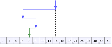
- lo=0, hi=6 → mid=3, a[3]=16. 16 < 23 → lo=4.
- lo=4, hi=6 → mid=5, a[5]=42. 42 > 23 → hi=4.
- lo=4, hi=4 → mid=4, a[4]=23. Found at index 4. Total: 3 comparisons for 7 elements (\( \lceil \log_2 7 \rceil = 3 \)).
- lo=0, hi=6 → mid=3, a[3]=16। 16 < 23 → lo=4।
- lo=4, hi=6 → mid=5, a[5]=42। 42 > 23 → hi=4।
- lo=4, hi=4 → mid=4, a[4]=23। Index 4-এ পাওয়া গেল। মোট: 7 element-এর জন্য 3 comparison (\( \lceil \log_2 7 \rceil = 3 \))।
- Array must be sorted — binary search on unsorted data gives wrong answers.
- Use
lo <= hi, notlo < hi, or you may miss the last element. mid = (lo + hi) / 2can overflow for big values; writelo + (hi - lo) / 2.- After comparing, move to
mid + 1ormid - 1. Keepingmidcan cause an infinite loop.
- Array অবশ্যই sorted হতে হবে — unsorted data-তে binary search ভুল উত্তর দেয়।
lo <= hiব্যবহার করুন,lo < hiনা, নাহলে শেষ element miss হতে পারে।- বড় value-তে
mid = (lo + hi) / 2overflow করতে পারে; লিখুনlo + (hi - lo) / 2। - Compare-এর পর
mid + 1বাmid - 1-এ যান।midরেখে দিলে infinite loop হতে পারে।
| Linear searchLinear search | Binary searchBinary search | |
|---|---|---|
| Needs sorted data?Sorted data লাগে? | Noনা | Yesহ্যাঁ |
| Worst timeWorst time | \( O(n) \) | \( O(\log n) \) |
| Best timeBest time | \( O(1) \) | \( O(1) \) |
| Works on linked list?Linked list-এ কাজ করে? | Yesহ্যাঁ | Not efficiently (no random access)ভালোভাবে না (random access নেই) |
4. Divide and Conquer4. Divide and Conquer
Divide and conquer is a 3-step pattern:
- Divide: break the problem into smaller subproblems of the same type.
- Conquer: solve each subproblem recursively (tiny ones directly).
- Combine: join the small answers into the full answer.
You already know two examples: merge sort (divide into halves, sort, merge) and binary search (divide, keep only one half, no combine needed). Quick sort is also divide and conquer (the work happens in the partition, before recursion).
Divide and conquer হলো 3-step pattern:
- Divide: problem-টাকে একই ধরনের ছোট ছোট subproblem-এ ভাঙুন।
- Conquer: প্রতিটা subproblem recursively solve করুন (খুব ছোট হলে সরাসরি)।
- Combine: ছোট উত্তরগুলো জোড়া দিয়ে পুরো উত্তর বানান।
দুটো example আপনি আগেই জানেন: merge sort (অর্ধেক করুন, sort করুন, merge করুন) আর binary search (divide করে শুধু এক অর্ধেক রাখুন, combine লাগে না)। Quick sort-ও divide and conquer (কাজটা হয় partition-এ, recursion-এর আগে)।
Example: fast power — power(x, n)Example: fast power — power(x, n)
Naive way: multiply \( x \) by itself \( n \) times → \( O(n) \). Divide and conquer way: \( x^n = (x^{n/2})^2 \) if \( n \) is even, and \( x \cdot (x^{(n-1)/2})^2 \) if odd. Only one recursive call!
সাধারণ উপায়: \( x \)-কে \( n \) বার গুণ → \( O(n) \)। Divide and conquer উপায়: \( n \) even হলে \( x^n = (x^{n/2})^2 \), odd হলে \( x \cdot (x^{(n-1)/2})^2 \)। মাত্র একটা recursive call!
long long power(long long x, int n) {
    if (n == 0) return 1;
    long long half = power(x, n / 2);
    if (n % 2 == 0) return half * half;
    else            return x * half * half;
}Example: max and min of an arrayExample: array-এর max আর min
Split the array in half, find (max, min) of each half recursively, then combine with 2 comparisons: overall max = max of two maxes, overall min = min of two mins. Recurrence: \( T(n) = 2T(n/2) + 2 \). This gives about \( 3n/2 - 2 \) comparisons, better than the naive \( 2n - 2 \) (comparing every element with both current max and min).
Array অর্ধেক করুন, প্রতিটা অর্ধেকের (max, min) recursively বের করুন, তারপর 2টা comparison দিয়ে combine করুন: মোট max = দুই max-এর বড়টা, মোট min = দুই min-এর ছোটটা। Recurrence: \( T(n) = 2T(n/2) + 2 \)। এতে প্রায় \( 3n/2 - 2 \) comparison লাগে, যা সাধারণ \( 2n - 2 \)-এর (প্রতিটা element-কে max আর min দুটোর সাথেই compare) চেয়ে ভালো।
5. Greedy Algorithms5. Greedy Algorithms
A greedy algorithm builds the answer step by step. At every step it takes the choice that looks best right now, and never goes back to change it. Greedy is simple and fast — but it only gives the correct answer for problems with a special structure (the "greedy choice" must be safe). For many problems, greedy is wrong.
Greedy algorithm উত্তরটা ধাপে ধাপে বানায়। প্রতিটা step-এ এই মুহূর্তে যেটা best দেখায় সেটাই নেয়, আর কখনো পিছনে গিয়ে বদলায় না। Greedy সহজ আর fast — কিন্তু শুধু বিশেষ structure-ওয়ালা problem-এ সঠিক উত্তর দেয় ("greedy choice" safe হতে হয়)। অনেক problem-এ greedy ভুল।
Activity selectionActivity selection
Problem: you have activities with start and finish times. One person can do one activity at a time. Pick the maximum number of non-overlapping activities. Greedy rule: sort by finish time, always take the activity that finishes earliest and does not clash with the last taken one.
Problem: কিছু activity আছে, প্রতিটার start আর finish time দেওয়া। একজন একসাথে একটাই activity করতে পারে। সর্বোচ্চ সংখ্যক non-overlapping activity বাছুন। Greedy rule: finish time দিয়ে sort করুন, সবসময় সেই activity নিন যেটা সবচেয়ে আগে শেষ হয় আর শেষ নেওয়াটার সাথে clash করে না।
- Sorted by finish: A(1,4), B(3,5), C(0,6), D(5,7), E(3,8), F(6,10), G(8,11).
- Take A (finishes first, at 4).
- B starts at 3 < 4 → clash, skip. C starts at 0 → clash, skip.
- D starts at 5 ≥ 4 → take D (finishes at 7).
- E starts 3 → skip. F starts 6 < 7 → skip.
- G starts 8 ≥ 7 → take G.
- Finish দিয়ে sorted: A(1,4), B(3,5), C(0,6), D(5,7), E(3,8), F(6,10), G(8,11)।
- A নিন (সবার আগে শেষ, 4-এ)।
- B শুরু 3 < 4 → clash, বাদ। C শুরু 0 → clash, বাদ।
- D শুরু 5 ≥ 4 → D নিন (শেষ 7-এ)।
- E শুরু 3 → বাদ। F শুরু 6 < 7 → বাদ।
- G শুরু 8 ≥ 7 → G নিন।
Coin change: where greedy works and where it failsCoin change: greedy কোথায় কাজ করে, কোথায় fail করে
Problem: make an amount with the fewest coins. Greedy rule: always take the biggest coin that fits.
- Works: coins {25, 10, 5, 1}, amount 63 → 25+25+10+1+1+1 = 6 coins. This is optimal (this coin system is "canonical").
- Fails: coins {1, 3, 4}, amount 6. Greedy: 4+1+1 = 3 coins. Optimal: 3+3 = 2 coins. Greedy got it wrong!
Lesson: greedy needs proof. When greedy fails, we use dynamic programming (next section).
Problem: সবচেয়ে কম coin দিয়ে একটা amount বানান। Greedy rule: সবসময় সবচেয়ে বড় coin নিন যেটা fit করে।
- কাজ করে: coin {25, 10, 5, 1}, amount 63 → 25+25+10+1+1+1 = 6 coin। এটাই optimal (এই coin system "canonical")।
- Fail করে: coin {1, 3, 4}, amount 6। Greedy: 4+1+1 = 3 coin। Optimal: 3+3 = 2 coin। Greedy ভুল করলো!
শিক্ষা: greedy-র জন্য proof লাগে। Greedy fail করলে আমরা dynamic programming ব্যবহার করি (পরের section)।
Huffman codingHuffman coding
Goal: compress text by giving short binary codes to frequent characters and longer codes to rare ones. Method: make each character a tree node with its frequency. Repeat: take the two nodes with the smallest frequencies, join them under a new parent whose frequency is their sum. Stop when one tree remains. Left edge = 0, right edge = 1. Each character's code = path from root. No code is a prefix of another (prefix-free), so decoding is unambiguous.
লক্ষ্য: বেশি frequent character-কে ছোট binary code আর কম frequent-কে লম্বা code দিয়ে text compress করা। পদ্ধতি: প্রতিটা character-কে frequency-সহ একটা tree node বানান। বারবার করুন: সবচেয়ে ছোট frequency-র দুটো node নিন, একটা নতুন parent-এর নিচে জোড়া দিন যার frequency হলো দুটোর যোগফল। একটা tree বাকি থাকলে থামুন। বাম edge = 0, ডান edge = 1। প্রতিটা character-এর code = root থেকে path। কোনো code অন্য code-এর prefix না (prefix-free), তাই decode করা unambiguous।
- Merge two smallest: a(5)+b(9) = node(14). Nodes: {12, 13, 14, 16, 45}
- Merge c(12)+d(13) = node(25). Nodes: {14, 16, 25, 45}
- Merge node14 + e(16) = node(30). Nodes: {25, 30, 45}
- Merge node25 + node30 = node(55). Nodes: {45, 55}
- Merge f(45) + node55 = root(100).
- সবচেয়ে ছোট দুটো merge: a(5)+b(9) = node(14)। Node: {12, 13, 14, 16, 45}
- c(12)+d(13) merge = node(25)। Node: {14, 16, 25, 45}
- node14 + e(16) merge = node(30)। Node: {25, 30, 45}
- node25 + node30 merge = node(55)। Node: {45, 55}
- f(45) + node55 merge = root(100)।

Bottlenecks / Limitations of Greedy (Real Exam!)Greedy-র Bottleneck / Limitation (Real Exam!)
Greedy is fast and simple, but it has clear weaknesses. The exam asks you to list the bottlenecks (limitations) of the greedy approach. Learn these five points:
- Local best ≠ global best. Greedy picks what looks best now. A chain of locally best choices can still end at a bad final answer (a local optimum, not the global optimum).
- No lookahead, no backtracking. Greedy never looks at future consequences, and once a choice is made it never goes back to undo it. One early wrong choice can ruin everything.
- Works only for special problems. The problem must have the greedy-choice property (a locally best choice is always safe) and optimal substructure (the best answer contains best answers of subproblems). Most problems do not have both.
- Correctness is hard to prove. Even when greedy is right, proving it (usually by an exchange argument) is tricky. A greedy that "looks right" can silently be wrong.
- Famous failures. Greedy fails on 0/1 knapsack (taking the best ratio item first can miss the optimal) and on coin change with a general coin system (coins {1, 3, 4}, amount 6: greedy gives 3 coins, optimal is 2). These need DP.
Greedy fast আর সহজ, কিন্তু এর স্পষ্ট কিছু দুর্বলতা আছে। পরীক্ষায় greedy approach-এর bottleneck (limitation) list করতে বলে। এই পাঁচটা point শিখুন:
- Local best ≠ global best। Greedy এই মুহূর্তে যা best দেখায় তাই নেয়। Locally best choice-এর chain শেষে একটা খারাপ answer-এ গিয়ে থামতে পারে (local optimum, global optimum না)।
- কোনো lookahead নেই, backtracking নেই। Greedy কখনো ভবিষ্যতের ফলাফল দেখে না, আর একবার choice নিলে ফিরে গিয়ে বদলায় না। শুরুর একটা ভুল choice সব নষ্ট করতে পারে।
- শুধু বিশেষ problem-এ কাজ করে। Problem-টার greedy-choice property (locally best choice সবসময় safe) আর optimal substructure (best answer-এর ভিতরে subproblem-এর best answer থাকে) — দুটোই থাকতে হয়। বেশিরভাগ problem-এ দুটো একসাথে থাকে না।
- Correctness প্রমাণ করা কঠিন। Greedy সঠিক হলেও তা প্রমাণ করা (সাধারণত exchange argument দিয়ে) কঠিন। "ঠিক মনে হচ্ছে" এমন greedy চুপচাপ ভুল হতে পারে।
- বিখ্যাত failure। Greedy fail করে 0/1 knapsack-এ (best ratio-র item আগে নিলে optimal miss হতে পারে) আর general coin system-এর coin change-এ (coin {1, 3, 4}, amount 6: greedy দেয় 3 coin, optimal 2)। এগুলোতে DP লাগে।
6. Dynamic Programming (DP)6. Dynamic Programming (DP)
DP solves problems that have two properties: overlapping subproblems (the same small problem appears many times) and optimal substructure (the best answer is built from best answers of subproblems). Trick: solve each subproblem once, save the result, reuse it.
- Memoization (top-down): write the normal recursion, but store each result in a table. Before computing, check the table first.
- Tabulation (bottom-up): fill a table from the smallest cases up to the answer, using loops. No recursion.
DP এমন problem solve করে যার দুটো property আছে: overlapping subproblems (একই ছোট problem বারবার আসে) আর optimal substructure (best উত্তরটা subproblem-গুলোর best উত্তর দিয়ে তৈরি হয়)। কৌশল: প্রতিটা subproblem একবারই solve করুন, result save করুন, আবার ব্যবহার করুন।
- Memoization (top-down): সাধারণ recursion লিখুন, কিন্তু প্রতিটা result একটা table-এ রাখুন। হিসাবের আগে আগে table check করুন।
- Tabulation (bottom-up): loop দিয়ে সবচেয়ে ছোট case থেকে উত্তর পর্যন্ত table fill করুন। কোনো recursion নেই।
Fibonacci: the classic first exampleFibonacci: classic প্রথম example
// Naive recursion: fib(n) = fib(n-1) + fib(n-2) → O(2^n), very slow
// fib(5) computes fib(3) twice, fib(2) three times... wasted work!

// Memoization (top-down): O(n)
long long memo[100]; // init all to -1
long long fib(int n) {
    if (n <= 1) return n;
    if (memo[n] != -1) return memo[n];   // already solved?
    return memo[n] = fib(n-1) + fib(n-2);
}

// Tabulation (bottom-up): O(n)
long long fibTab(int n) {
    long long dp[100];
    dp[0] = 0; dp[1] = 1;
    for (int i = 2; i <= n; i++) dp[i] = dp[i-1] + dp[i-2];
    return dp[n];
}
Naive recursion is \( O(2^n) \) because the same values are computed again and again. DP computes each fib(i) once → \( O(n) \).
সাধারণ recursion \( O(2^n) \) কারণ একই value বারবার হিসাব হয়। DP প্রতিটা fib(i) একবারই হিসাব করে → \( O(n) \)।
0/1 Knapsack0/1 Knapsack
Problem: a bag holds weight W. Each item has a weight and a value. Take each item fully or not at all (0/1). Maximize total value. DP: let dp[i][w] = best value using the first \( i \) items with capacity \( w \).
Problem: একটা bag-এ W weight ধরে। প্রতিটা item-এর weight আর value আছে। প্রতিটা item পুরোটা নিন বা একদমই না (0/1)। মোট value maximize করুন। DP: dp[i][w] = প্রথম \( i \)-টা item আর capacity \( w \) দিয়ে best value।
First choice = skip item \( i \). Second choice = take it (only if \( weight_i \le w \)).
প্রথম option = item \( i \) বাদ দিন। দ্বিতীয় option = নিন (শুধু যদি \( weight_i \le w \) হয়)।
| dp | w=0 | w=1 | w=2 | w=3 | w=4 | w=5 |
|---|---|---|---|---|---|---|
| no itemsকোনো item না | 0 | 0 | 0 | 0 | 0 | 0 |
| I1 (1,10) | 0 | 10 | 10 | 10 | 10 | 10 |
| +I2 (3,40) | 0 | 10 | 10 | 40 | 50 | 50 |
| +I3 (4,50) | 0 | 10 | 10 | 40 | 50 | 60 |
Sample cells: dp[2][4] = max(skip I2 → 10, take I2 → 40 + dp[1][1] = 40+10 = 50) = 50. dp[3][5] = max(skip I3 → 50, take I3 → 50 + dp[2][1] = 50+10 = 60) = 60. Answer: 60 (take I1 and I3). Complexity: \( O(nW) \).
কিছু cell-এর হিসাব: dp[2][4] = max(I2 বাদ → 10, I2 নিন → 40 + dp[1][1] = 40+10 = 50) = 50। dp[3][5] = max(I3 বাদ → 50, I3 নিন → 50 + dp[2][1] = 50+10 = 60) = 60। উত্তর: 60 (I1 আর I3 নিন)। Complexity: \( O(nW) \)।
Longest Common Subsequence (LCS)Longest Common Subsequence (LCS)
A subsequence keeps order but can skip characters. LCS of two strings = the longest subsequence present in both. DP: dp[i][j] = LCS length of first \( i \) chars of X and first \( j \) chars of Y.
Subsequence order ঠিক রাখে কিন্তু character skip করতে পারে। দুটো string-এর LCS = দুটোতেই থাকা সবচেয়ে লম্বা subsequence। DP: dp[i][j] = X-এর প্রথম \( i \) আর Y-এর প্রথম \( j \) character-এর LCS length।
| "" | B | D | C | B | |
|---|---|---|---|---|---|
| "" | 0 | 0 | 0 | 0 | 0 |
| A | 0 | 0 | 0 | 0 | 0 |
| B | 0 | 1 | 1 | 1 | 1 |
| C | 0 | 1 | 1 | 2 | 2 |
| B | 0 | 1 | 1 | 2 | 3 |
Answer: LCS length = 3 ("BCB"). Match cells (like B-B, C-C) take diagonal + 1; others take max of top and left. Complexity: \( O(mn) \).
উত্তর: LCS length = 3 ("BCB")। Match হওয়া cell (যেমন B-B, C-C) নেয় diagonal + 1; বাকিরা নেয় উপরের আর বামের max। Complexity: \( O(mn) \)।
Coin change with DP (fixes greedy!)DP দিয়ে coin change (greedy-র ভুল ঠিক করে!)
dp[v] = minimum coins to make amount \( v \). Base: dp[0] = 0. For each amount, try every coin:
dp[v] = amount \( v \) বানাতে minimum coin। Base: dp[0] = 0। প্রতিটা amount-এর জন্য প্রতিটা coin try করুন:
- dp[0]=0, dp[1]=1 (1), dp[2]=2 (1+1), dp[3]=1 (3), dp[4]=1 (4)
- dp[5] = 1 + min(dp[4], dp[2], dp[1]) = 1 + 1 = 2 (4+1)
- dp[6] = 1 + min(dp[5], dp[3], dp[2]) = 1 + dp[3] = 2 (3+3)
- dp[0]=0, dp[1]=1 (1), dp[2]=2 (1+1), dp[3]=1 (3), dp[4]=1 (4)
- dp[5] = 1 + min(dp[4], dp[2], dp[1]) = 1 + 1 = 2 (4+1)
- dp[6] = 1 + min(dp[5], dp[3], dp[2]) = 1 + dp[3] = 2 (3+3)
Greedy vs DPGreedy vs DP
| Greedy | DP | |
|---|---|---|
| ChoicesChoice | One "best now" choice, never revisitedএকটাই "এখন best" choice, আর ফেরা হয় না | Tries all choices, keeps the bestসব choice try করে, best-টা রাখে |
| CorrectnessCorrectness | Only for special problems (needs proof)শুধু বিশেষ problem-এ (proof লাগে) | Always correct if subproblems defined rightSubproblem ঠিকমতো define করলে সবসময় সঠিক |
| SpeedSpeed | Usually fasterসাধারণত বেশি fast | Slower, uses table memoryএকটু slow, table-এর memory লাগে |
| ExamplesExample | Activity selection, Huffman, Dijkstra, Prim, Kruskal | Knapsack 0/1, LCS, coin change (general), Bellman-Ford |
7. Graph Algorithms7. Graph Algorithms
BFS and DFSBFS আর DFS
BFS (Breadth-First Search) visits the graph level by level, using a queue. It first sees all neighbours, then neighbours of neighbours. DFS (Depth-First Search) goes as deep as possible along one path, then backtracks, using a stack (or recursion).
BFS (Breadth-First Search) graph-টা level by level ঘোরে, একটা queue ব্যবহার করে। আগে সব neighbour দেখে, তারপর neighbour-দের neighbour। DFS (Depth-First Search) এক path ধরে যত গভীরে যাওয়া যায় যায়, তারপর backtrack করে, একটা stack (বা recursion) ব্যবহার করে।
// BFS from source s (adjacency list, n nodes)
void bfs(int s) {
    queue<int> q;
    visited[s] = 1; q.push(s);
    while (!q.empty()) {
        int u = q.front(); q.pop();
        printf("%d ", u);                 // visit u
        for (int v : adj[u])              // all neighbours
            if (!visited[v]) { visited[v] = 1; q.push(v); }
    }
}

// DFS (recursive)
void dfs(int u) {
    visited[u] = 1;
    printf("%d ", u);                     // visit u
    for (int v : adj[u])
        if (!visited[v]) dfs(v);
}- Visit 1. Queue: [2, 3]
- Pop 2, visit. Its new neighbours: 4, 5. Queue: [3, 4, 5]
- Pop 3, visit. 4 already queued. Queue: [4, 5]
- Pop 4, visit. Pop 5, visit.
DFS trace from 1: visit 1 → go 2 → go 4 (2's smallest unvisited) → go 3 (4's neighbour) → backtrack to 4 → go 5. DFS order: 1, 2, 4, 3, 5.
- 1 visit। Queue: [2, 3]
- 2 pop, visit। এর নতুন neighbour: 4, 5। Queue: [3, 4, 5]
- 3 pop, visit। 4 আগেই queue-তে। Queue: [4, 5]
- 4 pop, visit। 5 pop, visit।
1 থেকে DFS trace: 1 visit → 2-তে যান → 4-এ যান (2-এর সবচেয়ে ছোট unvisited) → 3-এ যান (4-এর neighbour) → 4-এ backtrack → 5-এ যান। DFS order: 1, 2, 4, 3, 5।
| BFS | DFS | |
|---|---|---|
| Data structureData structure | Queue | Stack / recursion |
| ComplexityComplexity | \( O(V + E) \) | \( O(V + E) \) |
| ApplicationsApplication | Shortest path in unweighted graph, level order, bipartite checkUnweighted graph-এ shortest path, level order, bipartite check | Cycle detection, topological sort, connected components, maze solvingCycle detection, topological sort, connected component, maze solve |
Topological sort (idea)Topological sort (idea)
For a directed acyclic graph (DAG): order the nodes so every edge goes from earlier to later. Think of courses with prerequisites — take a course only after its prerequisites. Two ways: (1) DFS: after finishing a node, push it on a stack; pop all at the end. (2) Kahn's algorithm: repeatedly remove a node with in-degree 0 (no incoming edges). A cycle makes topological sort impossible. Example: edges 5→2, 5→0, 4→0, 4→1, 2→3, 3→1 → one valid order: 5, 4, 2, 3, 1, 0.
Directed acyclic graph (DAG)-এর জন্য: node-গুলো এমনভাবে সাজান যেন প্রতিটা edge আগের node থেকে পরের node-এ যায়। Prerequisite-ওয়ালা course-এর মতো ভাবুন — আগে prerequisite, তারপর course। দুই উপায়: (1) DFS: একটা node শেষ হলে stack-এ push করুন; শেষে সব pop করুন। (2) Kahn's algorithm: বারবার in-degree 0 (কোনো incoming edge নেই) এমন node সরান। Cycle থাকলে topological sort সম্ভব না। Example: edge 5→2, 5→0, 4→0, 4→1, 2→3, 3→1 → একটা valid order: 5, 4, 2, 3, 1, 0।
Dijkstra's algorithm (single-source shortest path)Dijkstra's algorithm (single-source shortest path)
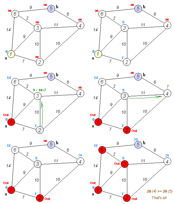
Finds shortest distances from one source to all nodes, when edge weights are non-negative. Greedy idea: keep a distance array. Repeatedly pick the unvisited node with the smallest distance, mark it final, and relax its edges (relax means: if dist[u] + w < dist[v], update dist[v]).
Edge weight non-negative হলে এক source থেকে সব node-এর shortest distance বের করে। Greedy idea: একটা distance array রাখুন। বারবার সবচেয়ে ছোট distance-ওয়ালা unvisited node নিন, তাকে final করুন, আর তার edge-গুলো relax করুন (relax মানে: dist[u] + w < dist[v] হলে dist[v] update)।
| StepStep | Picked nodeনেওয়া node | dist[A] | dist[B] | dist[C] | dist[D] | What happenedকী হলো |
|---|---|---|---|---|---|---|
| 0 | — | 0 | ∞ | ∞ | ∞ | initialশুরু |
| 1 | A (0) | 0 | 4 | 1 | ∞ | relax A–B: 0+4; A–C: 0+1relax A–B: 0+4; A–C: 0+1 |
| 2 | C (1) | 0 | 3 | 1 | 9 | relax C–B: 1+2=3 < 4 → update; C–D: 1+8=9relax C–B: 1+2=3 < 4 → update; C–D: 1+8=9 |
| 3 | B (3) | 0 | 3 | 1 | 8 | relax B–D: 3+5=8 < 9 → updaterelax B–D: 3+5=8 < 9 → update |
| 4 | D (8) | 0 | 3 | 1 | 8 | doneশেষ |
Final shortest distances from A: B = 3 (path A→C→B), C = 1, D = 8 (path A→C→B→D). Note how the direct edge A–B (4) lost to the path through C (3).
A থেকে final shortest distance: B = 3 (path A→C→B), C = 1, D = 8 (path A→C→B→D)। লক্ষ করুন সরাসরি A–B edge (4) হেরে গেল C-এর ভেতর দিয়ে path-এর (3) কাছে।
Bellman-Ford (handles negative weights)Bellman-Ford (negative weight সামলায়)
Idea: relax every edge, and repeat this \( V-1 \) times. Any shortest path has at most \( V-1 \) edges, so after \( V-1 \) rounds all distances are correct — even with negative edges. Bonus: run one extra round; if any distance still improves, the graph has a negative cycle (then "shortest path" has no meaning). Complexity: \( O(VE) \) — slower than Dijkstra, but safer.
Idea: প্রতিটা edge relax করুন, আর এটা \( V-1 \) বার repeat করুন। যেকোনো shortest path-এ সর্বোচ্চ \( V-1 \)-টা edge থাকে, তাই \( V-1 \) round পরে সব distance সঠিক — negative edge থাকলেও। Bonus: আরো এক round চালান; কোনো distance এখনো কমলে graph-এ negative cycle আছে (তখন "shortest path"-এর কোনো মানে নেই)। Complexity: \( O(VE) \) — Dijkstra-র চেয়ে slow, কিন্তু safe।
- Run Bellman-Ford from A. \( V-1 = 2 \) normal rounds finish. Say dist[A]=0, dist[B]=1, dist[C]=−2 after them.
- Now run one extra (the \( V \)-th) relaxation pass. Edge C→A: dist[C] + 1 = −2 + 1 = −1 < dist[A] = 0. A distance still improved!
- Rule: after \( V-1 \) rounds, all correct shortest distances are final. So if any edge still relaxes in the extra pass → a negative cycle is reachable → report "no valid shortest path". If nothing improves → no negative cycle, distances are safe.
- A থেকে Bellman-Ford চালান। \( V-1 = 2 \)-টা normal round শেষ হলো। ধরুন তখন dist[A]=0, dist[B]=1, dist[C]=−2।
- এবার আরো একটা extra (\( V \)-তম) relaxation pass চালান। Edge C→A: dist[C] + 1 = −2 + 1 = −1 < dist[A] = 0। একটা distance এখনো কমলো!
- নিয়ম: \( V-1 \) round-এর পর সব সঠিক shortest distance final হয়ে যায়। তাই extra pass-এ কোনো edge relax হলে → reachable negative cycle আছে → বলুন "valid shortest path নেই"। কিছু না কমলে → negative cycle নেই, distance-গুলো safe।
Minimum Spanning Tree (MST): Prim and KruskalMinimum Spanning Tree (MST): Prim আর Kruskal
A spanning tree connects all \( V \) nodes using exactly \( V-1 \) edges, with no cycle. The minimum spanning tree has the smallest total edge weight. Both famous algorithms are greedy:
- Prim: grow one tree. Start from any node; repeatedly add the cheapest edge that connects the tree to a new node.
- Kruskal: sort all edges by weight. Take edges smallest first, but skip any edge that makes a cycle. Stop after \( V-1 \) edges.
Spanning tree সব \( V \)-টা node-কে ঠিক \( V-1 \)-টা edge দিয়ে connect করে, কোনো cycle ছাড়া। Minimum spanning tree-র মোট edge weight সবচেয়ে কম। দুটো বিখ্যাত algorithm-ই greedy:
- Prim: একটা tree বড় করুন। যেকোনো node থেকে শুরু; বারবার সবচেয়ে সস্তা edge-টা নিন যা tree-কে একটা নতুন node-এর সাথে connect করে।
- Kruskal: সব edge weight দিয়ে sort করুন। ছোট থেকে edge নিন, কিন্তু cycle বানায় এমন edge বাদ দিন। \( V-1 \)-টা edge হলে থামুন।
Kruskal: sorted edges: A–C(1), C–B(2), A–B(4), B–D(5), C–D(8).
- Take A–C (1). Take C–B (2).
- A–B (4)? A and B already connected (A–C–B) → cycle → skip.
- Take B–D (5). Now 3 edges = V−1 → stop.
Prim (start A): cheapest edge from {A} is A–C (1) → add C. Cheapest from {A,C}: C–B (2) → add B. Cheapest from {A,C,B}: B–D (5) → add D. Same MST, weight 8. (Prim and Kruskal always give the same total weight.)
Kruskal: sorted edge: A–C(1), C–B(2), A–B(4), B–D(5), C–D(8)।
- A–C (1) নিন। C–B (2) নিন।
- A–B (4)? A আর B আগেই connected (A–C–B) → cycle → বাদ।
- B–D (5) নিন। এখন 3টা edge = V−1 → থামুন।
Prim (A থেকে শুরু): {A} থেকে সবচেয়ে সস্তা edge A–C (1) → C যোগ। {A,C} থেকে সস্তা: C–B (2) → B যোগ। {A,C,B} থেকে সস্তা: B–D (5) → D যোগ। একই MST, weight 8। (Prim আর Kruskal সবসময় একই মোট weight দেয়।)

DSU (Disjoint Set Union) — how Kruskal detects cyclesDSU (Disjoint Set Union) — Kruskal যেভাবে cycle ধরে
DSU (also called Union-Find) keeps track of groups. Two operations: find(x) — which group is x in (follow parents to the root)? union(x, y) — merge two groups. In Kruskal, before taking edge (u, v): if find(u) == find(v) they are already connected, so the edge would make a cycle → skip. Otherwise take the edge and union them. With "path compression" and "union by rank", each operation is almost \( O(1) \). Kruskal total: \( O(E \log E) \) (for sorting).
DSU (Union-Find-ও বলে) group-এর হিসাব রাখে। দুটো operation: find(x) — x কোন group-এ (parent ধরে root পর্যন্ত যান)? union(x, y) — দুটো group merge করুন। Kruskal-এ edge (u, v) নেওয়ার আগে: find(u) == find(v) হলে তারা আগেই connected, মানে edge-টা cycle বানাবে → বাদ। নাহলে edge নিন আর union করুন। "Path compression" আর "union by rank" দিলে প্রতিটা operation প্রায় \( O(1) \)। Kruskal মোট: \( O(E \log E) \) (sorting-এর জন্য)।
int parent[N];
int find(int x) {
    if (parent[x] == x) return x;
    return parent[x] = find(parent[x]);   // path compression
}
void unite(int x, int y) { parent[find(x)] = find(y); }Critical Path in a Task Graph (Real Exam!)Task Graph-এ Critical Path (Real Exam!)
Imagine a project made of tasks. Each task has a duration, and some tasks must wait for others (dependencies). Tasks with no dependency between them can run in parallel. The whole setup is a DAG (directed acyclic graph): task = node, dependency = edge.
The critical path is the longest path through this DAG (sum of task durations along the path). Key fact: the minimum possible completion time of the whole project = length of the critical path. Why? Every task on that path must run one after another — no parallelism can shorten it. Every other task can fit alongside.
How to find it — forward pass in topological order:
- Earliest Start (ES) of a task = max of Earliest Finish of all its dependencies (0 if none).
- Earliest Finish (EF) = ES + duration.
- Minimum completion time = max EF over all tasks. The critical path is the chain of tasks that produces this max.
ধরুন একটা project অনেকগুলো task দিয়ে তৈরি। প্রতিটা task-এর একটা duration আছে, আর কিছু task-কে অন্য task-এর জন্য অপেক্ষা করতে হয় (dependency)। যাদের মধ্যে dependency নেই, তারা parallel-এ চলতে পারে। পুরো ব্যাপারটা একটা DAG (directed acyclic graph): task = node, dependency = edge।
Critical path হলো এই DAG-এর ভিতর দিয়ে longest path (path-এর task duration-গুলোর যোগফল)। মূল কথা: পুরো project-এর minimum possible completion time = critical path-এর length। কেন? ওই path-এর প্রতিটা task একটার পর একটা চলতেই হবে — কোনো parallelism এটা ছোট করতে পারে না। বাকি সব task পাশে পাশে চলে যায়।
কীভাবে বের করবেন — topological order-এ forward pass:
- একটা task-এর Earliest Start (ES) = তার সব dependency-র Earliest Finish-এর max (dependency না থাকলে 0)।
- Earliest Finish (EF) = ES + duration।
- Minimum completion time = সব task-এর মধ্যে max EF। যে task-এর chain এই max বানায়, সেটাই critical path।
| Task | Duration | Depends on |
|---|---|---|
| A | 3 | — |
| B | 2 | — |
| C | 4 | A |
| D | 2 | A, B |
| E | 3 | D |
| F | 2 | C, E |
- A: ES = 0, EF = 0 + 3 = 3
- B: ES = 0, EF = 0 + 2 = 2
- C: ES = EF(A) = 3, EF = 3 + 4 = 7
- D: ES = max(EF(A), EF(B)) = max(3, 2) = 3, EF = 3 + 2 = 5
- E: ES = EF(D) = 5, EF = 5 + 3 = 8
- F: ES = max(EF(C), EF(E)) = max(7, 8) = 8, EF = 8 + 2 = 10
| Task | Duration | Depends on |
|---|---|---|
| A | 3 | — |
| B | 2 | — |
| C | 4 | A |
| D | 2 | A, B |
| E | 3 | D |
| F | 2 | C, E |
- A: ES = 0, EF = 0 + 3 = 3
- B: ES = 0, EF = 0 + 2 = 2
- C: ES = EF(A) = 3, EF = 3 + 4 = 7
- D: ES = max(EF(A), EF(B)) = max(3, 2) = 3, EF = 3 + 2 = 5
- E: ES = EF(D) = 5, EF = 5 + 3 = 8
- F: ES = max(EF(C), EF(E)) = max(7, 8) = 8, EF = 8 + 2 = 10
8. P, NP and Hard Problems (Real Exam Topic!)8. P, NP আর Hard Problems (Real Exam Topic!)
Some problems are easy for computers. Some are (probably) very hard. Complexity theory puts problems into classes. BUET has directly asked to define these classes and to draw their relationship diagram. Learn the four names below very well.
কিছু problem computer-এর জন্য সহজ। কিছু (সম্ভবত) খুবই কঠিন। Complexity theory problem-গুলোকে class-এ ভাগ করে। BUET সরাসরি এই class-গুলোর definition আর relationship diagram আঁকতে বলেছে। নিচের চারটা নাম খুব ভালো করে শিখুন।
Class P (Polynomial time)Class P (Polynomial time)
P = the set of problems a computer can solve in polynomial time — meaning time like \( O(n) \), \( O(n^2) \), \( O(n^3) \). These are the "easy" (tractable) problems.
- Examples: sorting an array (\( O(n \log n) \)), searching, shortest path with Dijkstra (\( O((V+E)\log V) \)), matrix multiplication.
P = সেই problem-গুলোর set যেগুলো computer polynomial time-এ solve করতে পারে — মানে \( O(n) \), \( O(n^2) \), \( O(n^3) \)-এর মতো time। এগুলো "সহজ" (tractable) problem।
- Example: array sort করা (\( O(n \log n) \)), searching, Dijkstra দিয়ে shortest path (\( O((V+E)\log V) \)), matrix multiplication।
Class NP (Nondeterministic Polynomial time)Class NP (Nondeterministic Polynomial time)
NP = the set of problems where, if someone gives you a solution, you can verify (check) it in polynomial time. Finding the solution may be hard, but checking is easy.
- Examples: SAT (given a true/false setting of variables, checking the formula is easy), TSP decision version ("is there a tour of length ≤ k?" — given a tour, adding up its length is easy), Sudoku (checking a filled board is easy).
- Every problem in P is also in NP — if you can solve it fast, you can surely check a given answer fast. So \( P \subseteq NP \).
NP = সেই problem-গুলোর set যেখানে কেউ আপনাকে একটা solution দিয়ে দিলে, আপনি সেটা polynomial time-এ verify (check) করতে পারেন। Solution খুঁজে বের করা কঠিন হতে পারে, কিন্তু check করা সহজ।
- Example: SAT (variable-গুলোর true/false মান দেওয়া থাকলে formula check করা সহজ), TSP decision version ("length ≤ k-এর কোনো tour আছে কি?" — tour দেওয়া থাকলে length যোগ করা সহজ), Sudoku (ভরা board check করা সহজ)।
- P-এর প্রতিটা problem NP-তেও আছে — fast solve করতে পারলে দেওয়া answer fast check-ও করতে পারবেন। তাই \( P \subseteq NP \)।
NP-Complete and NP-HardNP-Complete আর NP-Hard
- NP-Complete = the hardest problems inside NP. A problem is NP-Complete if (1) it is in NP, and (2) every problem in NP can be converted (reduced) to it in polynomial time. Solve one NP-Complete problem fast → you solve ALL of NP fast. Examples: SAT (the first one, by Cook's theorem), 3-SAT, TSP decision version, vertex cover, graph coloring, subset sum.
- NP-Hard = at least as hard as every problem in NP, but it does not have to be in NP itself (its answer may not even be checkable fast, or it may not be a yes/no problem). Examples: TSP optimization version ("find the shortest tour" — even checking that a tour is the shortest is hard), the halting problem (not solvable at all!).
- Relationship: NP-Complete = NP ∩ NP-Hard. NP-Complete problems are exactly the NP-Hard problems that also sit inside NP.
- NP-Complete = NP-এর ভেতরের সবচেয়ে কঠিন problem। একটা problem NP-Complete হয় যদি (1) এটা NP-তে থাকে, আর (2) NP-এর প্রতিটা problem-কে polynomial time-এ এটাতে convert (reduce) করা যায়। একটা NP-Complete problem fast solve করলে → পুরো NP fast solve হয়ে যায়। Example: SAT (প্রথমটা, Cook's theorem দিয়ে), 3-SAT, TSP decision version, vertex cover, graph coloring, subset sum।
- NP-Hard = NP-এর প্রতিটা problem-এর মতো বা তার চেয়েও কঠিন, কিন্তু নিজে NP-তে থাকা জরুরি না (এর answer fast check-ও করা নাও যেতে পারে, বা এটা yes/no problem নাও হতে পারে)। Example: TSP optimization version ("সবচেয়ে ছোট tour বের করুন" — একটা tour-ই যে সবচেয়ে ছোট, সেটা check করাও কঠিন), halting problem (আদৌ solve-ই করা যায় না!)।
- Relationship: NP-Complete = NP ∩ NP-Hard। NP-Hard problem-গুলোর মধ্যে যেগুলো NP-এর ভেতরেও আছে, সেগুলোই NP-Complete।
The relationship diagram (BUET asked to draw this!)Relationship diagram (BUET এটা আঁকতে বলেছে!)
Read the diagram like this: P sits inside NP. NP-Hard sticks out to the right — part of it is inside NP, part is outside. The overlap of NP and NP-Hard is exactly NP-Complete. If P = NP were true, the picture would collapse: P, NP and NP-Complete would all become one same set (and NP-Hard would contain that whole set).
Diagram-টা এভাবে পড়ুন: P থাকে NP-এর ভেতরে। NP-Hard ডান দিকে বেরিয়ে আছে — এর কিছু অংশ NP-এর ভেতরে, কিছু বাইরে। NP আর NP-Hard-এর overlap-টাই হলো NP-Complete। যদি P = NP সত্যি হতো, ছবিটা ভেঙে পড়ত: P, NP আর NP-Complete সব একই set হয়ে যেত (আর NP-Hard পুরো set-টাকে ধারণ করত)।
P vs NP — the biggest open questionP vs NP — সবচেয়ে বড় open question
Is P = NP? In words: if an answer is easy to check, is it also easy to find? Nobody knows. It is the most famous open problem in computer science, with a $1 million Clay Millennium Prize. Most researchers believe P ≠ NP — that is why we draw the diagram above with P as a strict smaller circle.
P = NP কি? সহজ কথায়: একটা answer যদি সহজে check করা যায়, তাহলে কি সেটা সহজে খুঁজেও বের করা যায়? কেউ জানে না। এটা computer science-এর সবচেয়ে বিখ্যাত open problem, $1 million Clay Millennium Prize আছে এর জন্য। বেশিরভাগ researcher বিশ্বাস করেন P ≠ NP — তাই উপরের diagram-এ P-কে ছোট আলাদা circle হিসেবে আঁকা হয়।
Approximation algorithm vs Heuristic algorithmApproximation algorithm vs Heuristic algorithm
NP-Hard problems have no known fast exact algorithm. So in practice we use two kinds of "good enough" methods. BUET asked the difference directly.
NP-Hard problem-এর জন্য কোনো fast exact algorithm জানা নেই। তাই বাস্তবে আমরা দুই ধরনের "good enough" পদ্ধতি ব্যবহার করি। BUET সরাসরি এদের পার্থক্য জিজ্ঞেস করেছে।
| Approximation algorithmApproximation algorithm | Heuristic algorithmHeuristic algorithm | |
|---|---|---|
| GuaranteeGuarantee | Has a provable (mathematical) bound on how far the answer can be from the optimal.Answer optimal থেকে সর্বোচ্চ কতদূর হতে পারে তার provable (mathematical) bound আছে। | No guarantee at all. It just works well in practice, usually.কোনো guarantee নেই। সাধারণত practice-এ ভালো কাজ করে, এটুকুই। |
| Answer qualityAnswer quality | Example: a 2-approximation for vertex cover always returns a cover at most 2× the optimal size — proven.Example: vertex cover-এর 2-approximation সবসময় optimal-এর সর্বোচ্চ 2× size-এর cover দেয় — proven। | Can be very good or very bad; on some inputs it may fail badly and we cannot predict when.খুব ভালো বা খুব খারাপ হতে পারে; কোনো কোনো input-এ ভীষণ খারাপ করতে পারে, কখন করবে বলা যায় না। |
| ExamplesExample | 2-approximation for vertex cover, Christofides' 1.5-approximation for metric TSP.Vertex cover-এর 2-approximation, metric TSP-র Christofides' 1.5-approximation। | A* search heuristics, hill climbing, genetic algorithms, greedy rules of thumb.A* search-এর heuristics, hill climbing, genetic algorithm, greedy rule of thumb। |
| One-line memory trickএক লাইনে মনে রাখার trick | "Approximation = promise on paper.""Approximation = কাগজে promise।" | "Heuristic = hope from experience.""Heuristic = অভিজ্ঞতা থেকে আশা।" |
Practice Questions (Admission Style)Practice Questions (Admission Style)
Show Answerউত্তর দেখুন
Show Answerউত্তর দেখুন
for (i = 0; i < n; i++)
    for (j = 0; j < i; j++)
sum++;for (i = 0; i < n; i++)
for (j = 0; j < i; j++)
sum++;Show Answerউত্তর দেখুন
Show Answerউত্তর দেখুন
Show Answerউত্তর দেখুন
Show Answerউত্তর দেখুন
Show Answerউত্তর দেখুন
Show Answerউত্তর দেখুন
Show Answerউত্তর দেখুন
- key = 4: 9 > 4 shifts right, insert 4 → [4, 9, 6, 2]
- key = 6: 9 > 6 shifts, 4 < 6 stop, insert 6 → [4, 6, 9, 2]
- key = 2: 9, 6, 4 all shift, insert 2 at front → [2, 4, 6, 9]
- key = 4: 9 > 4 ডানে shift, 4 insert → [4, 9, 6, 2]
- key = 6: 9 > 6 shift, 4 < 6 থামুন, 6 insert → [4, 6, 9, 2]
- key = 2: 9, 6, 4 সব shift, 2 সামনে insert → [2, 4, 6, 9]
Show Answerউত্তর দেখুন
- Step 1: lo=0, hi=8, mid=4 → a[4]=27. 27 < 31 → lo = 5.
- Step 2: lo=5, hi=8, mid=6 → a[6]=33. 33 > 31 → hi = 5.
- Step 3: lo=5, hi=5, mid=5 → a[5]=31. Found at index 5.
- Step 1: lo=0, hi=8, mid=4 → a[4]=27। 27 < 31 → lo = 5।
- Step 2: lo=5, hi=8, mid=6 → a[6]=33। 33 > 31 → hi = 5।
- Step 3: lo=5, hi=5, mid=5 → a[5]=31। Index 5-এ পাওয়া গেল।
Show Answerউত্তর দেখুন
- j=0: 4 < 3? No. j=1: 9 < 3? No.
- j=2: 2 < 3? Yes → i=0, swap a[0],a[2] → [2, 9, 4, 7, 3]
- j=3: 7 < 3? No.
- Final: swap pivot into i+1 = 1 → [2, 3, 4, 7, 9]. Pivot 3 is fixed at index 1.
- j=0: 4 < 3? না। j=1: 9 < 3? না।
- j=2: 2 < 3? হ্যাঁ → i=0, a[0],a[2] swap → [2, 9, 4, 7, 3]
- j=3: 7 < 3? না।
- শেষে: pivot-কে i+1 = 1-এ swap → [2, 3, 4, 7, 9]। Pivot 3 index 1-এ fix।
Show Answerউত্তর দেখুন
dp = [0, 1, 2, 3, 4, 1, 1, 2, 3, 4, 2]
Key cells: dp[5]=1 (coin 5), dp[6]=1 (coin 6), dp[10] = 1 + min(dp[9]=4, dp[5]=1, dp[4]=4) = 1 + 1 = 2 coins (5+5). Greedy (5 coins) is far from optimal (2 coins) — this coin system is not canonical, so DP is required.
dp = [0, 1, 2, 3, 4, 1, 1, 2, 3, 4, 2]
গুরুত্বপূর্ণ cell: dp[5]=1 (coin 5), dp[6]=1 (coin 6), dp[10] = 1 + min(dp[9]=4, dp[5]=1, dp[4]=4) = 1 + 1 = 2 coin (5+5)। Greedy (5 coin) optimal (2 coin) থেকে অনেক দূরে — এই coin system canonical না, তাই DP লাগবে।
Show Answerউত্তর দেখুন
- Merge 1: p(10) + q(15) = n1(25). Left: {25, 30, 45}
- Merge 2: n1(25) + r(30) = n2(55). Left: {45, 55}
- Merge 3: s(45) + n2(55) = root(100).
Total bits = 45·1 + 30·2 + 10·3 + 15·3 = 45 + 60 + 30 + 45 = 180 bits. (Fixed 2-bit codes would need 100·2 = 200 bits, so Huffman saves 20.)
- Merge 1: p(10) + q(15) = n1(25)। বাকি: {25, 30, 45}
- Merge 2: n1(25) + r(30) = n2(55)। বাকি: {45, 55}
- Merge 3: s(45) + n2(55) = root(100)।
মোট bit = 45·1 + 30·2 + 10·3 + 15·3 = 45 + 60 + 30 + 45 = 180 bit। (Fixed 2-bit code-এ লাগত 100·2 = 200 bit, তাই Huffman বাঁচালো 20।)
Show Answerউত্তর দেখুন
| dp | 0 | 1 | 2 | 3 | 4 |
|---|---|---|---|---|---|
| no items | 0 | 0 | 0 | 0 | 0 |
| A (2,3) | 0 | 0 | 3 | 3 | 3 |
| +B (3,4) | 0 | 0 | 3 | 4 | 4 |
| +C (1,2) | 0 | 2 | 3 | 5 | 6 |
Max value = 6. Backtrack: C was taken (6 ≠ 4), left w = 3; B row at w=3 is 4 ≠ dp[A][3]=3 so B taken, left w = 0; A not taken. Chosen items: B and C (weight 3+1 = 4, value 4+2 = 6).
| dp | 0 | 1 | 2 | 3 | 4 |
|---|---|---|---|---|---|
| কোনো item না | 0 | 0 | 0 | 0 | 0 |
| A (2,3) | 0 | 0 | 3 | 3 | 3 |
| +B (3,4) | 0 | 0 | 3 | 4 | 4 |
| +C (1,2) | 0 | 2 | 3 | 5 | 6 |
Max value = 6। Backtrack: C নেওয়া হয়েছে (6 ≠ 4), বাকি w = 3; w=3-এ B row-এর 4 ≠ dp[A][3]=3 তাই B নেওয়া, বাকি w = 0; A নেওয়া হয়নি। নেওয়া item: B আর C (weight 3+1 = 4, value 4+2 = 6)।
Show Answerউত্তর দেখুন
- Init: dist[S]=0, A=∞, B=∞, C=∞.
- Pick S(0): relax S–A → A=7; S–B → B=2.
- Pick B(2): relax B–A → 2+3=5 < 7 → A=5; B–C → 2+8=10 → C=10.
- Pick A(5): relax A–C → 5+1=6 < 10 → C=6.
- Pick C(6): done.
Kruskal: sorted edges A–C(1), S–B(2), B–A(3), S–A(7), B–C(8). Take A–C(1), S–B(2), B–A(3) — no cycles, 3 edges = V−1 → stop. MST weight = 1+2+3 = 6. Edges: {A–C, S–B, B–A}.
Yes — here they use the same edges. But this is a coincidence, not a rule: shortest-path trees and MSTs optimize different things and often differ.
- শুরু: dist[S]=0, A=∞, B=∞, C=∞।
- S(0) নিন: relax S–A → A=7; S–B → B=2।
- B(2) নিন: relax B–A → 2+3=5 < 7 → A=5; B–C → 2+8=10 → C=10।
- A(5) নিন: relax A–C → 5+1=6 < 10 → C=6।
- C(6) নিন: শেষ।
Kruskal: sorted edge A–C(1), S–B(2), B–A(3), S–A(7), B–C(8)। A–C(1), S–B(2), B–A(3) নিন — কোনো cycle নেই, 3টা edge = V−1 → থামুন। MST weight = 1+2+3 = 6। Edge: {A–C, S–B, B–A}।
হ্যাঁ — এখানে edge-গুলো একই। কিন্তু এটা কাকতালীয়, নিয়ম না: shortest-path tree আর MST আলাদা জিনিস optimize করে, প্রায়ই আলাদা হয়।
Show Answerউত্তর দেখুন
- P = problems that can be solved in polynomial time (like \( O(n^2) \)). Example: sorting an array.
- NP = problems whose given solution can be verified in polynomial time (finding it may be hard, checking is easy). Example: SAT — checking a given true/false assignment is easy.
- NP-Complete = problems that are in NP AND every NP problem reduces to them in polynomial time (the hardest inside NP). Example: 3-SAT.
- NP-Hard = at least as hard as everything in NP, but not required to be in NP. Example: TSP optimization, halting problem.
- P = যে problem polynomial time-এ (যেমন \( O(n^2) \)) solve করা যায়। Example: array sort করা।
- NP = যে problem-এর দেওয়া solution polynomial time-এ verify করা যায় (খুঁজে বের করা কঠিন হতে পারে, check করা সহজ)। Example: SAT — দেওয়া true/false assignment check করা সহজ।
- NP-Complete = যে problem NP-তে আছে এবং NP-এর প্রতিটা problem polynomial time-এ এতে reduce হয় (NP-এর ভেতরের সবচেয়ে কঠিন)। Example: 3-SAT।
- NP-Hard = NP-এর সবকিছুর মতো বা তার চেয়ে কঠিন, কিন্তু NP-তে থাকা জরুরি না। Example: TSP optimization, halting problem।
Show Answerউত্তর দেখুন
Show Answerউত্তর দেখুন
Show Answerউত্তর দেখুন
- T1: ES = 0, EF = 0 + 4 = 4
- T2: ES = 0, EF = 0 + 3 = 3
- T3: ES = EF(T1) = 4, EF = 4 + 5 = 9
- T4: ES = max(EF(T1), EF(T2)) = max(4, 3) = 4, EF = 4 + 2 = 6
- T5: ES = max(EF(T3), EF(T4)) = max(9, 6) = 9, EF = 9 + 4 = 13
- T1: ES = 0, EF = 0 + 4 = 4
- T2: ES = 0, EF = 0 + 3 = 3
- T3: ES = EF(T1) = 4, EF = 4 + 5 = 9
- T4: ES = max(EF(T1), EF(T2)) = max(4, 3) = 4, EF = 4 + 2 = 6
- T5: ES = max(EF(T3), EF(T4)) = max(9, 6) = 9, EF = 9 + 4 = 13