Data StructuresData Structures

How we store data so we can find it, add it, and remove it fast. This is the heart of CSE admission exams. Data কীভাবে রাখলে দ্রুত খোঁজা, যোগ করা আর মুছে ফেলা যায় — সেটাই data structure। CSE admission exam-এর সবচেয়ে গুরুত্বপূর্ণ অংশ এটা।

In this chapterএই chapter-এ যা আছে

Arrays and Linked ListsArrays এবং Linked Lists
StackStack
QueueQueue
Trees and Binary Search Tree (BST)Trees এবং Binary Search Tree (BST)
HeapHeap
HashingHashing
Graph RepresentationsGraph Representations
Practice QuestionsPractice Questions

1. Arrays and Linked Lists1. Arrays এবং Linked Lists

Array: data in one continuous blockArray: এক টানা memory block-এ data

An array stores elements side by side in memory. All elements have the same type and size. Because the block is continuous, the computer can jump to any index with simple math. This is why array access is \( O(1) \).

Array element গুলোকে memory-তে পাশাপাশি রাখে। সব element-এর type আর size একই। Memory block টানা (contiguous) বলে computer সহজ অঙ্ক করে যেকোনো index-এ সরাসরি যেতে পারে। এজন্যই array access \( O(1) \)।

\[ \text{address}(A[i]) = \text{base address} + i \times \text{size of one element} \]

Example (index math): An int array starts at address 2000. Each int is 4 bytes. Where is A[5]?
Address = 2000 + 5 × 4 = 2020.
For a 2D array A[R][C] stored row-major (like C): address of A[i][j] = base + (i × C + j) × size. So for int A[10][20] at base 1000, A[3][4] is at 1000 + (3×20 + 4)×4 = 1000 + 256 = 1256.

Example (index math): একটা int array শুরু হয়েছে address 2000-এ। প্রতিটা int = 4 bytes। A[5] কোথায়?
Address = 2000 + 5 × 4 = 2020।
2D array A[R][C] row-major-এ (C language-এর মতো) থাকলে: A[i][j]-এর address = base + (i × C + j) × size। যেমন int A[10][20], base 1000 হলে A[3][4] = 1000 + (3×20 + 4)×4 = 1000 + 256 = 1256।

Array weakness: inserting or deleting in the middle needs shifting. To insert at position 0 of an array with \( n \) items, we shift all \( n \) items right. That is \( O(n) \). Also, a normal array has fixed size.

Array-এর দুর্বলতা: মাঝখানে insert বা delete করতে element shift করতে হয়। \( n \) item-এর array-তে position 0-তে insert করতে হলে সব \( n \) item ডানে সরাতে হয়। এটা \( O(n) \)। আর সাধারণ array-এর size fixed।

Linked list: nodes connected by pointersLinked list: pointer দিয়ে জোড়া node

A linked list stores data in separate nodes. Each node holds the data and a pointer to the next node. Nodes can live anywhere in memory. So the list can grow and shrink easily. But to reach the 100th node, we must walk through 99 nodes first — access is \( O(n) \).

Linked list data রাখে আলাদা আলাদা node-এ। প্রতিটা node-এ থাকে data আর পরের node-এর pointer। Node গুলো memory-র যেকোনো জায়গায় থাকতে পারে। তাই list সহজে বড়-ছোট হতে পারে। কিন্তু 100 নম্বর node-এ যেতে হলে আগের 99টা node পার হতে হয় — access \( O(n) \)।

Singly linked list diagram — A singly linked list. Each node points to the next. The last node points to NULL. Singly linked list। প্রতিটা node পরেরটাকে point করে। শেষ node point করে NULL-এ।

Three common kinds:

Singly linked list: each node has one pointer, next. We can only move forward.
Doubly linked list: each node has next and prev. We can move both ways. Deleting a known node is easy, but each node needs extra memory.
Circular linked list: the last node points back to the first node instead of NULL. Useful for round-robin tasks.

তিনটা common ধরন:

Singly linked list: প্রতিটা node-এ একটাই pointer, next। শুধু সামনে যাওয়া যায়।
Doubly linked list: প্রতিটা node-এ next আর prev দুটোই থাকে। দুই দিকেই যাওয়া যায়। কোনো node জানা থাকলে delete করা সহজ, কিন্তু প্রতি node-এ বাড়তি memory লাগে।
Circular linked list: শেষ node NULL-এর বদলে প্রথম node-কে point করে। Round-robin কাজে কাজে লাগে।

Doubly linked list diagram — A doubly linked list. Each node points forward and backward. Doubly linked list। প্রতিটা node সামনে ও পেছনে point করে।

C code: insert and delete in a singly linked listC code: singly linked list-এ insert এবং delete

struct Node {
    int data;
    struct Node *next;
};

/* Insert at the front: O(1) */
struct Node* insertFront(struct Node *head, int value) {
    struct Node *n = (struct Node*) malloc(sizeof(struct Node));
    n->data = value;
    n->next = head;   /* new node points to old head */
    return n;         /* new node becomes the head */
}

/* Insert after a given node p: O(1) */
void insertAfter(struct Node *p, int value) {
    struct Node *n = (struct Node*) malloc(sizeof(struct Node));
    n->data = value;
    n->next = p->next;
    p->next = n;
}

/* Delete the first node with given value: O(n) to find it */
struct Node* deleteValue(struct Node *head, int value) {
    if (head == NULL) return NULL;
    if (head->data == value) {          /* case 1: delete head */
        struct Node *t = head->next;
        free(head);
        return t;
    }
    struct Node *cur = head;
    while (cur->next != NULL && cur->next->data != value)
        cur = cur->next;
    if (cur->next != NULL) {            /* case 2: found in middle/end */
        struct Node *t = cur->next;
        cur->next = t->next;            /* skip over the node */
        free(t);
    }
    return head;
}

Exam tip: The order of pointer changes matters. In insertAfter, if you write p->next = n; before n->next = p->next;, you lose the rest of the list. BUET loves "what is wrong with this code" questions on this.

Exam tip: Pointer বদলানোর order খুব গুরুত্বপূর্ণ। insertAfter-এ যদি আগে p->next = n; লেখো, তারপর n->next = p->next;, তাহলে list-এর বাকি অংশ হারিয়ে যাবে। BUET-এ "এই code-এ ভুল কী" ধরনের প্রশ্ন এখান থেকে আসে।

Insert into a Sorted Linked ListSorted Linked List-এ Insert

Very common exam task: the list is already sorted (ascending), and we must insert a new value so the list stays sorted. The trick is to walk with two pointers — prev and curr — and stop as soon as curr's data is not smaller than the new value. Then the new node goes between prev and curr. Two cases need care:

Head insert: the list is empty, or the new value is smaller than the head → the new node becomes the new head.
Middle / tail insert: walk until curr is NULL (tail) or curr->data >= value (middle), then re-link.

Exam-এর খুব common কাজ: list আগে থেকেই sorted (ascending), নতুন একটা value এমনভাবে insert করতে হবে যেন list sorted-ই থাকে। কৌশলটা হলো দুইটা pointer — prev আর curr — দিয়ে হাঁটা, আর যেই curr-এর data নতুন value-র চেয়ে ছোট না হয়, সেখানেই থামা। তখন নতুন node বসবে prev আর curr-এর মাঝে। দুইটা case-এ সাবধান:

Head insert: list খালি, বা নতুন value head-এর চেয়ে ছোট → নতুন node-ই নতুন head হবে।
Middle / tail insert: curr NULL হওয়া (tail) বা curr->data >= value হওয়া (middle) পর্যন্ত হাঁটো, তারপর re-link করো।

/* insert value into an ascending sorted list; returns the (maybe new) head */
struct Node* sortedInsert(struct Node *head, int value) {
    struct Node *n = malloc(sizeof(struct Node));
    n->data = value;
    n->next = NULL;

    /* case 1: empty list, or new value goes before the head */
    if (head == NULL || value < head->data) {
        n->next = head;
        return n;                     /* n is the new head */
    }

    /* case 2: prev/curr walk to find the spot (middle or tail) */
    struct Node *prev = head, *curr = head->next;
    while (curr != NULL && curr->data < value) {
        prev = curr;
        curr = curr->next;
    }
    n->next = curr;                   /* curr may be NULL: tail insert */
    prev->next = n;                   /* link n after prev */
    return head;                      /* head did not change */
}

Trace: insert 25 into 10 → 20 → 30 → 40.
Step 1: 25 < 10? No → not a head insert.
Step 2: prev = 10, curr = 20. Is 20 < 25? Yes → move up: prev = 20, curr = 30.
Step 3: Is 30 < 25? No → stop here.
Step 4: n->next = curr (25 → 30), then prev->next = n (20 → 25).
Result: 10 → 20 → 25 → 30 → 40. Sorted, as promised.
Check the edge cases too: inserting 5 hits case 1 (new head: 5 → 10 → ...); inserting 50 walks until curr = NULL and lands at the tail (... → 40 → 50). Time: \( O(n) \) — one walk, no extra space.

Trace: 10 → 20 → 30 → 40 list-এ 25 insert করি।
Step 1: 25 < 10? না → head insert নয়।
Step 2: prev = 10, curr = 20। 20 < 25? হ্যাঁ → এগোও: prev = 20, curr = 30।
Step 3: 30 < 25? না → এখানেই থামো।
Step 4: n->next = curr (25 → 30), তারপর prev->next = n (20 → 25)।
Result: 10 → 20 → 25 → 30 → 40। Sorted-ই আছে।
Edge case গুলোও দেখো: 5 insert করলে case 1 লাগে (নতুন head: 5 → 10 → ...); 50 insert করলে curr = NULL পর্যন্ত হেঁটে tail-এ বসে (... → 40 → 50)। Time: \( O(n) \) — একবার হাঁটা, extra space নেই।

Note: This exact question — write a function to insert a number into a sorted linked list — was asked in the BUET MSc admission exam (October 2017). Write it with pointer notation (p->next), no array brackets, and always show the head-insert case separately.

Note: ঠিক এই প্রশ্নটাই — sorted linked list-এ একটা number insert করার function লেখো — BUET MSc admission exam-এ এসেছিল (October 2017)। Pointer notation (p->next) দিয়ে লেখো, কোনো array bracket নয়, আর head-insert case টা সবসময় আলাদা করে দেখাও।

Array vs linked listArray vs linked list

Operation / propertyOperation / property	Array	Singly linked listSingly linked list
Access by indexIndex দিয়ে access	\( O(1) \)	\( O(n) \)
Search (unsorted)Search (unsorted)	\( O(n) \)	\( O(n) \)
Insert / delete at frontসামনে insert / delete	\( O(n) \) (shift all)(সব shift করতে হয়)	\( O(1) \)
Insert / delete in middle (position known)মাঝে insert / delete (position জানা)	\( O(n) \)	\( O(1) \) (after reaching the node)(node-এ পৌঁছানোর পরে)
Memory layoutMemory layout	Contiguous, cache friendlyContiguous, cache friendly	Scattered, extra pointer per nodeছড়ানো, প্রতি node-এ বাড়তি pointer
SizeSize	Fixed (static array)Fixed (static array)	Grows and shrinks easilyসহজে বাড়ে-কমে

Cycle Detection — Floyd's Tortoise and HareCycle Detection — Floyd's Tortoise and Hare

Sometimes a linked list has a problem: the last node does not point to NULL. Instead it points back to some earlier node. This makes a cycle (loop). If we walk the list with one pointer, we go round and round forever. Floyd's algorithm finds a cycle using two pointers:

slow (the tortoise) moves 1 step at a time.
fast (the hare) moves 2 steps at a time.
If fast reaches NULL → the list ends normally → no cycle.
If slow and fast ever land on the same node → there is a cycle.

Time: \( O(n) \). Extra space: \( O(1) \) — only two pointers. That is why exams love this answer.

কখনো কখনো linked list-এ একটা সমস্যা থাকে: শেষ node NULL-কে point করে না। বরং আগের কোনো node-কে point করে। এতে একটা cycle (loop) তৈরি হয়। এক pointer দিয়ে হাঁটলে আমরা চিরকাল ঘুরতেই থাকব। Floyd's algorithm দুইটা pointer দিয়ে cycle খুঁজে বের করে:

slow (tortoise) একবারে 1 step যায়।
fast (hare) একবারে 2 step যায়।
fast যদি NULL-এ পৌঁছায় → list স্বাভাবিকভাবে শেষ → cycle নেই।
slow আর fast যদি কখনো একই node-এ পড়ে → cycle আছে।

Time: \( O(n) \)। Extra space: \( O(1) \) — মাত্র দুইটা pointer। এজন্যই exam-এ এই উত্তরটা এত প্রিয়।

/* returns 1 if the list has a cycle, 0 if it ends at NULL */
int hasCycle(struct Node *head) {
    struct Node *slow = head, *fast = head;
    while (fast != NULL && fast->next != NULL) {
        slow = slow->next;            /* 1 step  */
        fast = fast->next->next;      /* 2 steps */
        if (slow == fast) return 1;   /* they met inside a cycle */
    }
    return 0;                         /* fast fell off the end: no cycle */
}

Why it works (simple argument): If there is no cycle, fast reaches NULL and we stop — easy. If there is a cycle, both pointers eventually enter it and go round and round. Inside the cycle, fast gains exactly 1 position on slow every step. So the gap between them shrinks by 1 each step. The gap must reach 0 before slow finishes even one full lap — so they are guaranteed to meet. The loop always ends.

কেন কাজ করে (সহজ যুক্তি): Cycle না থাকলে fast NULL-এ পৌঁছে যায়, আমরা থেমে যাই — সহজ। Cycle থাকলে দুই pointer-ই একসময় cycle-এর ভিতরে ঢুকে ঘুরতে থাকে। Cycle-এর ভিতরে fast প্রতি step-এ slow-এর থেকে ঠিক 1 position এগোয়। তাই তাদের মধ্যের gap প্রতি step-এ 1 করে কমে। slow এক চক্কর শেষ করার আগেই gap 0 হয়ে যায় — মানে তারা মিলবেই। Loop সবসময় শেষ হয়।

Example (the snake vs snail problem): You are given a linked list. It is either a "snake" (a normal list — walking it ends at NULL) or a "snail" (a circular list — the tail points back into the list, so walking never ends). Give an algorithm to tell which one it is.
Answer approach: Run Floyd's two-pointer walk: each round, slow = slow->next and fast = fast->next->next. If fast or fast->next becomes NULL → the list terminates → it is a snake. If slow == fast at some point → the two pointers met inside a loop → it is a snail. Time \( O(n) \), extra space \( O(1) \). (A simpler answer — remembering every visited node in a hash table — also works but needs \( O(n) \) extra space. Mention that Floyd is better.)

Example (snake vs snail problem): তোমাকে একটা linked list দেওয়া হলো। এটা হয় "snake" (সাধারণ list — হাঁটলে NULL-এ শেষ হয়) নয়তো "snail" (circular list — tail আবার list-এর ভিতরে point করে, তাই হাঁটা কখনো শেষ হয় না)। কোনটা, সেটা বের করার algorithm দাও।
Answer approach: Floyd's two-pointer walk চালাও: প্রতি round-এ slow = slow->next আর fast = fast->next->next। fast বা fast->next NULL হয়ে গেলে → list শেষ হয় → এটা snake। কোনো এক সময় slow == fast হলে → pointer দুটো loop-এর ভিতরে মিলে গেছে → এটা snail। Time \( O(n) \), extra space \( O(1) \)। (সহজ আরেকটা উত্তর — প্রতিটা visited node hash table-এ রাখা — সেটাও চলে, কিন্তু \( O(n) \) extra space লাগে। বলে দাও Floyd better।)

Note: This exact snake/snail question was asked in the BUET MSc admission exam (April 2024). Learn the two-pointer walk and the one-line reason why the pointers must meet.

Note: এই snake/snail প্রশ্নটাই BUET MSc admission exam-এ এসেছিল (April 2024)। Two-pointer walk আর "pointer দুটো মিলবেই কেন" — এই এক লাইনের যুক্তিটা শিখে রাখো।

2. Stack2. Stack

A stack is a LIFO (Last In, First Out) structure. Think of a pile of plates. You put a new plate on top. You also take a plate from the top. The last plate you put is the first one you take.

Main operations, all \( O(1) \):

push(x) — put x on top.
pop() — remove and return the top item.
peek() (or top()) — look at the top item without removing it.
isEmpty() — check if the stack has no items.

Pushing into a full array stack causes overflow. Popping an empty stack causes underflow.

Stack হলো LIFO (Last In, First Out) structure। প্লেটের স্তূপের মতো। নতুন প্লেট উপরে রাখো, নেওয়ার সময়ও উপর থেকে নাও। শেষে যেটা রেখেছো, সেটাই আগে বের হয়।

মূল operation, সবগুলোই \( O(1) \):

push(x) — x-কে উপরে রাখা।
pop() — উপরের item সরিয়ে ফেরত দেওয়া।
peek() (বা top()) — না সরিয়ে উপরের item দেখা।
isEmpty() — stack খালি কি না দেখা।

Full array stack-এ push করলে overflow হয়। খালি stack-এ pop করলে underflow হয়।

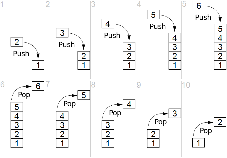
Stack push and pop diagram — Push adds to the top. Pop removes from the top. Only the top is touched. Push উপরে যোগ করে, pop উপর থেকে সরায়। শুধু top নিয়েই কাজ হয়।

Array implementationArray implementation

#define MAX 100
int stack[MAX];
int top = -1;                 /* empty stack */

void push(int x) {
    if (top == MAX - 1) { printf("Overflow\n"); return; }
    stack[++top] = x;         /* move top up, then store */
}

int pop(void) {
    if (top == -1) { printf("Underflow\n"); return -1; }
    return stack[top--];      /* return item, then move top down */
}

int peek(void) { return stack[top]; }

Linked list implementationLinked list implementation

Push = insert at the head. Pop = delete the head. Both are \( O(1) \), and there is no fixed size limit.

Push মানে head-এ insert। Pop মানে head delete। দুটোই \( O(1) \), আর size-এর কোনো fixed limit নেই।

struct Node { int data; struct Node *next; };
struct Node *top = NULL;

void push(int x) {
    struct Node *n = (struct Node*) malloc(sizeof(struct Node));
    n->data = x;
    n->next = top;
    top = n;
}

int pop(void) {
    if (top == NULL) return -1;   /* underflow */
    int v = top->data;
    struct Node *t = top;
    top = top->next;
    free(t);
    return v;
}

Application 1: balanced parenthesesApplication 1: balanced parentheses

To check if brackets like {[()]} are balanced: scan left to right. Push every opening bracket. For every closing bracket, pop and check that it matches. At the end, the stack must be empty.

{[()]}-এর মতো bracket balanced কি না দেখতে: বাম থেকে ডানে scan করো। প্রতিটা opening bracket push করো। প্রতিটা closing bracket-এ pop করে match কি না দেখো। শেষে stack খালি থাকতে হবে।

Example: Check {[(]}. Push {, push [, push (. Next char is ] — pop gives (, but ( does not match ]. So it is not balanced.

Example: {[(]} check করি। Push {, push [, push (। পরের character ] — pop করলে পাই (, কিন্তু ( আর ] match করে না। তাই এটা balanced নয়।

Application 2: infix to postfix conversionApplication 2: infix থেকে postfix conversion

Infix: A + B (operator between operands). Postfix: A B + (operator after operands). Computers like postfix because no parentheses are needed. Conversion rules (shunting-yard idea):

Operand → output it directly.
( → push it.
) → pop and output until ( is found; discard both parentheses.
Operator → pop and output all stack operators with higher or equal precedence, then push the new operator. (Precedence: ^ > * / > + -. ^ is right-associative, so for ^ pop only strictly higher.)
End of input → pop everything to output.

Infix: A + B (operator মাঝে)। Postfix: A B + (operator পরে)। Computer postfix পছন্দ করে কারণ parentheses লাগে না। Conversion-এর নিয়ম:

Operand → সরাসরি output-এ।
( → push।
) → ( পাওয়া পর্যন্ত pop করে output-এ দাও; দুই parentheses-ই বাদ।
Operator → stack-এ থাকা higher বা equal precedence-এর operator গুলো pop করে output-এ দাও, তারপর নতুন operator push করো। (Precedence: ^ > * / > + -। ^ right-associative, তাই ^-এর ক্ষেত্রে শুধু strictly higher হলে pop।)
Input শেষ → stack-এর সব pop করে output-এ।

Full worked example: Convert A + B * (C - D) to postfix.

Symbol	Stack (bottom→top)	Output
A	(empty)	A
+	+	A
B	+	A B
*	+ *	A B ( * has higher precedence than +, so just push )
(	+ * (	A B
C	+ * (	A B C
-	+ * ( -	A B C
D	+ * ( -	A B C D
)	+ *	A B C D - ( pop until "(" )
end	(empty)	*A B C D - +**

Answer: A B C D - * +

পূর্ণ worked example: A + B * (C - D)-কে postfix-এ convert করি।

Symbol	Stack (নিচ→উপর)	Output
A	(খালি)	A
+	+	A
B	+	A B
*	+ *	A B ( *-এর precedence + থেকে বেশি, তাই শুধু push )
(	+ * (	A B
C	+ * (	A B C
-	+ * ( -	A B C
D	+ * ( -	A B C D
)	+ *	A B C D - ( "(" পাওয়া পর্যন্ত pop )
শেষ	(খালি)	*A B C D - +**

উত্তর: A B C D - * +

Example (postfix evaluation): Evaluate 6 2 3 + - 3 *. Push 6, 2, 3. See +: pop 3, 2 → 2+3=5, push 5. See -: pop 5, 6 → 6−5=1, push 1. Push 3. See *: pop 3, 1 → 1×3=3. Note: for - and /, the first popped value is the right operand.

Example (postfix evaluation): 6 2 3 + - 3 * evaluate করি। Push 6, 2, 3। + পেলে: pop 3, 2 → 2+3=5, push 5। - পেলে: pop 5, 6 → 6−5=1, push 1। Push 3। * পেলে: pop 3, 1 → 1×3=3। খেয়াল রাখো: - আর /-এর ক্ষেত্রে প্রথমে pop হওয়া value-টা right operand।

Application 3: function call stackApplication 3: function call stack

When a program calls a function, the computer pushes a "frame" (return address, local variables) on the call stack. When the function returns, its frame is popped. Recursion works because of this. Too-deep recursion fills the stack — that is a stack overflow. Other uses: undo feature, browser back button, DFS.

Program কোনো function call করলে computer একটা "frame" (return address, local variable) call stack-এ push করে। Function return করলে frame pop হয়। Recursion এই ভাবেই কাজ করে। বেশি গভীর recursion হলে stack ভরে যায় — সেটাই stack overflow। আরও ব্যবহার: undo feature, browser-এর back button, DFS।

Application 4: palindrome check with a stack and a queueApplication 4: stack আর queue দিয়ে palindrome check

Example (exam question): Write pseudocode to check if a string is a palindrome (reads the same forwards and backwards, like MADAM) using one stack and one queue.
Idea: Push every character on a stack AND enqueue it in a queue. The stack gives the string back reversed (LIFO); the queue gives it back in order (FIFO). If both outputs match character by character, the string equals its own reverse — a palindrome.

Example (exam question): একটা string palindrome কি না (সামনে-পেছনে একই পড়া যায়, যেমন MADAM) — একটা stack আর একটা queue দিয়ে check করার pseudocode লেখো।
Idea: প্রতিটা character stack-এ push করো এবং queue-তে enqueue করো। Stack string-টা উল্টো করে ফেরত দেয় (LIFO); queue ঠিক order-এ ফেরত দেয় (FIFO)। দুটোর output character ধরে ধরে মিলে গেলে string টা তার নিজের reverse-এর সমান — মানে palindrome।

isPalindrome(s):
    S = empty stack, Q = empty queue
    for each character c in s:
        push(S, c)                       // S will return s reversed
        enqueue(Q, c)                    // Q will return s in order
    while S is not empty:
        if pop(S) != dequeue(Q):
            return FALSE                 // mismatch: not a palindrome
    return TRUE                          // all matched

Trace with MADAM: pop order = M A D A M, dequeue order = M A D A M — all 5 pairs match → palindrome. With BUET: first pair is pop = T vs dequeue = B → mismatch → not a palindrome. Time \( O(n) \), space \( O(n) \).

MADAM দিয়ে trace: pop order = M A D A M, dequeue order = M A D A M — 5টা pair-ই মিলে যায় → palindrome। BUET দিয়ে: প্রথম pair-এ pop = T আর dequeue = B → মিলল না → palindrome নয়। Time \( O(n) \), space \( O(n) \)।

Note: This stack + queue palindrome question was asked in the BUET MSc admission exam (April 2017). The key sentence for full marks: "stack reverses the order, queue keeps the order."

Note: এই stack + queue palindrome প্রশ্নটা BUET MSc admission exam-এ এসেছিল (April 2017)। Full marks-এর key লাইন: "stack order উল্টে দেয়, queue order ঠিক রাখে।"

3. Queue3. Queue

A queue is a FIFO (First In, First Out) structure. Like a line at a ticket counter. New people join at the rear. Service happens at the front. The person who came first leaves first.

enqueue(x) — add x at the rear. \( O(1) \)
dequeue() — remove the item at the front. \( O(1) \)
front() — look at the front item.

Queue হলো FIFO (First In, First Out) structure। টিকিট কাউন্টারের লাইনের মতো। নতুন মানুষ ঢোকে rear-এ, service হয় front-এ। যে আগে এসেছে, সে আগে বের হয়।

enqueue(x) — rear-এ x যোগ করা। \( O(1) \)
dequeue() — front-এর item সরানো। \( O(1) \)
front() — front-এর item দেখা।

Circular queue: reusing empty spaceCircular queue: খালি জায়গা আবার ব্যবহার

In a simple array queue, after many dequeues the front part of the array becomes wasted. A circular queue fixes this: when the index reaches the end, it wraps around to 0 using modulo. With array size \( N \):

সাধারণ array queue-তে অনেকবার dequeue-এর পর array-র সামনের অংশ waste হয়ে যায়। Circular queue এটা ঠিক করে: index শেষে পৌঁছালে modulo দিয়ে আবার 0-তে ঘুরে আসে। Array size \( N \) হলে:

\[ \text{rear} = (\text{rear} + 1) \bmod N, \qquad \text{front} = (\text{front} + 1) \bmod N \]

#define N 5
int q[N];
int front = 0, count = 0;      /* count-based version: simplest */

void enqueue(int x) {
    if (count == N) { printf("Full\n"); return; }
    q[(front + count) % N] = x;
    count++;
}

int dequeue(void) {
    if (count == 0) { printf("Empty\n"); return -1; }
    int v = q[front];
    front = (front + 1) % N;
    count--;
    return v;
}

Exam tip (the full/empty trick): If we keep only front and rear pointers (no count), then "full" and "empty" can look the same. The standard trick: keep one slot always unused.
Empty: front == rear.
Full: (rear + 1) % N == front.
So a circular queue of array size N holds at most N − 1 items in this scheme. BUET asks this a lot.

Exam tip (full/empty trick): শুধু front আর rear pointer রাখলে (count ছাড়া) "full" আর "empty" একই রকম দেখায়। Standard trick: একটা slot সবসময় খালি রাখা।
Empty: front == rear।
Full: (rear + 1) % N == front।
তাই এই scheme-এ array size N-এর circular queue-তে সর্বোচ্চ N − 1 item রাখা যায়। BUET-এ এটা প্রায়ই আসে।

Example (trace): N = 5, front = rear = 0. Enqueue 10, 20, 30, 40 → rear becomes 4, queue holds 4 items — now (4+1)%5 == 0 == front, so it is full (one slot wasted). Dequeue twice → front = 2. Enqueue 50 → stored at index 4, rear = 0 (wrapped around!). Items in order: 30, 40, 50.

Example (trace): N = 5, front = rear = 0। Enqueue 10, 20, 30, 40 → rear হয় 4, queue-তে 4টা item — এখন (4+1)%5 == 0 == front, তাই এটা full (একটা slot waste)। দুইবার dequeue → front = 2। Enqueue 50 → index 4-এ বসে, rear = 0 (ঘুরে গেল!)। Item-এর order: 30, 40, 50।

Queue with a singly linked list: O(1) enqueue AND dequeueSingly linked list দিয়ে queue: O(1) enqueue এবং dequeue

Example (exam question): How can a queue built on a singly linked list give \( O(1) \) enqueue AND \( O(1) \) dequeue?
Answer: Keep two pointers: front (first node) and rear (last node). Then enqueue at the rear, dequeue at the front. Both touch only one end directly — no walking needed.

Example (exam question): Singly linked list দিয়ে বানানো queue কীভাবে \( O(1) \) enqueue এবং \( O(1) \) dequeue দুটোই দিতে পারে?
Answer: দুইটা pointer রাখো: front (প্রথম node) আর rear (শেষ node)। তারপর rear-এ enqueue, front-এ dequeue করো। দুটো operation-ই সরাসরি এক প্রান্তে কাজ করে — কোনো হাঁটাহাঁটি লাগে না।

struct Node { int data; struct Node *next; };
struct Node *front = NULL, *rear = NULL;

void enqueue(int x) {                     /* O(1): attach at rear */
    struct Node *n = (struct Node*) malloc(sizeof(struct Node));
    n->data = x; n->next = NULL;
    if (rear == NULL) { front = rear = n; return; }  /* empty queue */
    rear->next = n;                       /* old last points to new */
    rear = n;                             /* new node is the rear   */
}

int dequeue(void) {                       /* O(1): detach at front */
    if (front == NULL) return -1;         /* empty */
    int v = front->data;
    struct Node *t = front;
    front = front->next;                  /* second node becomes front */
    if (front == NULL) rear = NULL;       /* queue became empty */
    free(t);
    return v;
}

Why does the reverse assignment fail? Suppose we enqueue at the front and dequeue at the rear. Enqueue at front is still \( O(1) \). But to dequeue at the rear, we must set rear to the node before the last one — and a singly linked list has no prev pointer. The only way to find that node is to walk from the front: \( O(n) \). So the assignment of ends is forced: remove where you can reach the next node (front), add where NULL goes (rear).

উল্টোটা করলে fail করে কেন? ধরো front-এ enqueue আর rear-এ dequeue করলাম। Front-এ enqueue তখনো \( O(1) \)। কিন্তু rear-এ dequeue করতে হলে rear-কে শেষের আগের node-এ আনতে হবে — আর singly linked list-এ কোনো prev pointer নেই। সেই node খুঁজতে front থেকে হেঁটে যাওয়া ছাড়া উপায় নেই: \( O(n) \)। তাই প্রান্ত বাছাই একটাই: যেখান থেকে পরের node ধরা যায় সেখানে remove (front), যেখানে NULL বসে সেখানে add (rear)।

Note: This exact question — O(1) enqueue and dequeue with a singly linked list — was asked in the BUET MSc admission exam (April 2019). Always mention BOTH pointers and why the reverse choice costs \( O(n) \).

Note: ঠিক এই প্রশ্নটাই — singly linked list দিয়ে O(1) enqueue আর dequeue — BUET MSc admission exam-এ এসেছিল (April 2019)। উত্তরে অবশ্যই দুইটা pointer-এর কথা আর উল্টো choice-এ কেন \( O(n) \) লাগে সেটা লিখবে।

Deque and priority queueDeque এবং priority queue

Deque (double-ended queue): insert and delete allowed at both ends. It can act as both a stack and a queue.
Priority queue: each item has a priority. Dequeue always removes the highest priority item, not the oldest one. Best implementation: a heap (Section 5), giving \( O(\log n) \) insert and delete.

Queue applications: CPU scheduling, printer jobs, BFS in graphs, buffering (keyboard, network packets).

Deque (double-ended queue): দুই প্রান্তেই insert আর delete করা যায়। এটা stack আর queue দুটোর মতোই কাজ করতে পারে।
Priority queue: প্রতিটা item-এর একটা priority থাকে। Dequeue সবসময় highest priority item সরায়, পুরনোটা নয়। Best implementation: heap (Section 5), যাতে insert আর delete \( O(\log n) \)।

Queue-এর ব্যবহার: CPU scheduling, printer job, graph-এ BFS, buffering (keyboard, network packet)।

4. Trees and Binary Search Tree (BST)4. Trees এবং Binary Search Tree (BST)

Tree terminologyTree terminology

A tree is a hierarchy of nodes with no cycles. Key words:

Root: the top node.
Parent / child: a node directly above / below another.
Leaf: a node with no children.
Edge: the link between a parent and a child. A tree with \( n \) nodes has exactly \( n - 1 \) edges.
Height: the longest path from the root down to a leaf (counted in edges).
Depth (level): distance of a node from the root. Root is at level 0.
Subtree: a node plus all nodes under it.

Tree হলো cycle ছাড়া node-এর একটা hierarchy। Key শব্দগুলো:

Root: সবচেয়ে উপরের node।
Parent / child: ঠিক উপরের / নিচের node।
Leaf: যে node-এর কোনো child নেই।
Edge: parent আর child-এর মধ্যের link। \( n \) node-এর tree-তে edge ঠিক \( n - 1 \)টা।
Height: root থেকে leaf পর্যন্ত সবচেয়ে লম্বা path (edge-এ গোনা)।
Depth (level): root থেকে node-এর দূরত্ব। Root থাকে level 0-তে।
Subtree: একটা node আর তার নিচের সব node।

Binary tree typesBinary tree-র ধরন

A binary tree gives each node at most 2 children (left and right).

Full binary tree: every node has 0 or 2 children (never exactly 1).
Complete binary tree: all levels are full, except maybe the last, which is filled from the left. (Heaps use this.)
Perfect binary tree: all levels are completely full. A perfect tree of height \( h \) has \( 2^{h+1} - 1 \) nodes and \( 2^h \) leaves.

Useful fact: a binary tree with height \( h \) has at most \( 2^h \) nodes at level \( h \). A binary tree with \( n \) nodes has height at least \( \lfloor \log_2 n \rfloor \).

Binary tree-তে প্রতিটা node-এর সর্বোচ্চ 2টা child থাকে (left আর right)।

Full binary tree: প্রতিটা node-এর child হয় 0টা নয় 2টা (কখনো ঠিক 1টা নয়)।
Complete binary tree: সব level পূর্ণ, শুধু শেষ level-টা হয়তো বাকি — আর সেটা বাম দিক থেকে ভরা। (Heap এটাই ব্যবহার করে।)
Perfect binary tree: সব level সম্পূর্ণ ভরা। Height \( h \)-এর perfect tree-তে node \( 2^{h+1} - 1 \)টা, leaf \( 2^h \)টা।

দরকারি fact: level \( h \)-এ সর্বোচ্চ \( 2^h \)টা node থাকতে পারে। \( n \) node-এর binary tree-র height কমপক্ষে \( \lfloor \log_2 n \rfloor \)।

Binary Search Tree (BST)Binary Search Tree (BST)

BST rule: for every node, all keys in the left subtree are smaller, and all keys in the right subtree are larger. This rule lets us search like binary search: at each node, go left or right and throw away half the tree (if balanced).

BST-র নিয়ম: প্রতিটা node-এর left subtree-র সব key তার থেকে ছোট, আর right subtree-র সব key বড়। এই নিয়মের জন্য binary search-এর মতো খোঁজা যায়: প্রতিটা node-এ left বা right-এ গিয়ে (balanced হলে) অর্ধেক tree বাদ দেওয়া যায়।

A BST. Left of 8: everything smaller (3, 1, 6, 4, 7). Right of 8: everything larger (10, 14). একটা BST। 8-এর left-এ সব ছোট (3, 1, 6, 4, 7)। 8-এর right-এ সব বড় (10, 14)।

Tree traversalsTree traversal

Preorder: Root → Left → Right. (Used to copy a tree.)
Inorder: Left → Root → Right. (On a BST this gives sorted order!)
Postorder: Left → Right → Root. (Used to delete a tree.)
Level order: level by level, top to bottom — done with a queue (BFS).

Preorder: Root → Left → Right। (Tree copy করতে কাজে লাগে।)
Inorder: Left → Root → Right। (BST-তে এটা দেয় sorted order!)
Postorder: Left → Right → Root। (Tree delete করতে কাজে লাগে।)
Level order: level ধরে ধরে, উপর থেকে নিচ — queue দিয়ে করা হয় (BFS)।

void inorder(struct Node *r) {
    if (r == NULL) return;
    inorder(r->left);
    printf("%d ", r->data);   /* move this line first for preorder,
                                 last for postorder */
    inorder(r->right);
}

Worked example: For the BST in the figure (8, 3, 10, 1, 6, 14, 4, 7):

Preorder: 8 3 1 6 4 7 10 14
Inorder: 1 3 4 6 7 8 10 14 ← sorted, as promised
Postorder: 1 4 7 6 3 14 10 8
Level order: 8 3 10 1 6 14 4 7

Worked example: ছবির BST-র জন্য (8, 3, 10, 1, 6, 14, 4, 7):

Preorder: 8 3 1 6 4 7 10 14
Inorder: 1 3 4 6 7 8 10 14 ← কথামতো sorted
Postorder: 1 4 7 6 3 14 10 8
Level order: 8 3 10 1 6 14 4 7

Building a tree from traversalsTraversal থেকে tree বানানো

Inorder alone cannot rebuild a tree. But inorder + preorder (or inorder + postorder) can. Method: the first item of preorder is the root. Find it in inorder — everything to its left is the left subtree, everything to its right is the right subtree. Repeat.

শুধু inorder দিয়ে tree বানানো যায় না। কিন্তু inorder + preorder (বা inorder + postorder) দিয়ে যায়। পদ্ধতি: preorder-এর প্রথম item-টাই root। সেটাকে inorder-এ খুঁজে বের করো — তার বামের সব হলো left subtree, ডানের সব right subtree। এভাবে repeat করো।

Example: Preorder = A B D E C F, Inorder = D B E A C F.
Root = A (first of preorder). In inorder, left of A = {D, B, E}, right of A = {C, F}.
Left part: preorder gives B next → B is root of left subtree. In D B E, D is left of B, E is right of B.
Right part: preorder gives C → root of right subtree. In C F, F is right of C.
Final tree: A(root), left = B with children D, E; right = C with right child F.

Example: Preorder = A B D E C F, Inorder = D B E A C F।
Root = A (preorder-এর প্রথম)। Inorder-এ A-এর বামে = {D, B, E}, ডানে = {C, F}।
Left অংশ: preorder-এ পরে আসে B → left subtree-র root B। D B E-তে D হলো B-র left, E হলো B-র right।
Right অংশ: preorder-এ C → right subtree-র root। C F-এ F হলো C-র right child।
Final tree: A(root), left = B (child D, E); right = C (right child F)।

BST insert and searchBST insert এবং search

struct Node* insert(struct Node *r, int key) {
    if (r == NULL) {                       /* empty spot found */
        struct Node *n = (struct Node*) malloc(sizeof(struct Node));
        n->data = key; n->left = n->right = NULL;
        return n;
    }
    if (key < r->data)      r->left  = insert(r->left,  key);
    else if (key > r->data) r->right = insert(r->right, key);
    return r;
}

struct Node* search(struct Node *r, int key) {
    if (r == NULL || r->data == key) return r;
    if (key < r->data) return search(r->left, key);
    return search(r->right, key);
}

Trace: insert 5, 3, 8, 1 into an empty BST.
Insert 5 → tree is empty, 5 becomes root.
Insert 3 → 3 < 5, go left. Left is empty → 3 becomes left child of 5.
Insert 8 → 8 > 5, go right. Right is empty → 8 becomes right child of 5.
Insert 1 → 1 < 5 go left, 1 < 3 go left again → 1 becomes left child of 3.
Inorder now: 1 3 5 8 (sorted ✓).

Trace: খালি BST-তে 5, 3, 8, 1 insert করি।
Insert 5 → tree খালি, 5 হলো root।
Insert 3 → 3 < 5, left-এ যাই। Left খালি → 3 হলো 5-এর left child।
Insert 8 → 8 > 5, right-এ যাই। Right খালি → 8 হলো 5-এর right child।
Insert 1 → 1 < 5 left, 1 < 3 আবার left → 1 হলো 3-এর left child।
এখন inorder: 1 3 5 8 (sorted ✓)।

BST delete: the 3 casesBST delete: 3টা case

Leaf node: just remove it.
One child: replace the node with its only child.
Two children: find the inorder successor (smallest node in the right subtree). Copy its value into the node. Then delete the successor (which has at most one child). The inorder predecessor (largest in left subtree) also works.

Leaf node: সরাসরি মুছে দাও।
একটা child: node-এর জায়গায় তার একমাত্র child বসাও।
দুইটা child: inorder successor খুঁজে বের করো (right subtree-র সবচেয়ে ছোট node)। তার value node-এ copy করো। তারপর successor-কে delete করো (তার সর্বোচ্চ একটা child থাকে)। Inorder predecessor (left subtree-র সবচেয়ে বড়) দিয়েও চলে।

Example: In the figure's BST, delete 3 (it has two children: 1 and 6). Right subtree of 3 is {6, 4, 7}; smallest there is 4. Copy 4 into 3's spot. Delete the old 4 (a leaf). New inorder: 1 4 6 7 8 10 14 — still sorted ✓.

Example: ছবির BST-তে 3 delete করি (তার দুই child: 1 আর 6)। 3-এর right subtree {6, 4, 7}; সেখানে সবচেয়ে ছোট 4। 3-এর জায়গায় 4 copy করো। পুরনো 4 (leaf) delete করো। নতুন inorder: 1 4 6 7 8 10 14 — এখনো sorted ✓।

Exam tip: For the two-children case, examiners check whether you know "inorder successor = leftmost node of the right subtree". Also remember: BST operations cost \( O(h) \) where \( h \) is the height. Balanced tree: \( h = O(\log n) \). Sorted-order inserts (1, 2, 3, 4, ...) make a "skewed" tree — basically a linked list — so \( h = n \) and everything becomes \( O(n) \). This worst case is a favorite exam question.

Exam tip: দুই-child case-এ examiner দেখতে চায় তুমি জানো কি না: "inorder successor = right subtree-র সবচেয়ে বাম node"। আরও মনে রাখো: BST operation-এর cost \( O(h) \), যেখানে \( h \) হলো height। Balanced tree হলে \( h = O(\log n) \)। Sorted order-এ insert করলে (1, 2, 3, 4, ...) tree "skewed" হয়ে যায় — আসলে একটা linked list — তখন \( h = n \), সব operation \( O(n) \)। এই worst case টা exam-এর প্রিয় প্রশ্ন।

Balanced trees: the AVL ideaBalanced tree: AVL-এর ধারণা

An AVL tree is a BST that keeps itself balanced. Rule: for every node, the heights of the left and right subtrees differ by at most 1 (balance factor ∈ {−1, 0, +1}). After each insert or delete, if a node breaks the rule, the tree fixes itself with rotations:

LL case (left-left heavy) → one right rotation.
RR case → one left rotation.
LR case → left rotation on the child, then right rotation on the node.
RL case → right rotation on the child, then left rotation on the node.

Result: height stays \( O(\log n) \), so search, insert, delete are all guaranteed \( O(\log n) \). Example: insert 1, 2, 3 into an AVL tree. After 3, node 1 is RR-heavy → left rotation → 2 becomes root with children 1 and 3.

AVL tree হলো এমন BST যেটা নিজেকে balanced রাখে। নিয়ম: প্রতিটা node-এ left আর right subtree-র height-এর পার্থক্য সর্বোচ্চ 1 (balance factor ∈ {−1, 0, +1})। Insert বা delete-এর পর কোনো node নিয়ম ভাঙলে tree নিজেকে ঠিক করে rotation দিয়ে:

LL case (left-left heavy) → একটা right rotation।
RR case → একটা left rotation।
LR case → child-এ left rotation, তারপর node-এ right rotation।
RL case → child-এ right rotation, তারপর node-এ left rotation।

ফলাফল: height থাকে \( O(\log n) \), তাই search, insert, delete সবই guaranteed \( O(\log n) \)। Example: AVL tree-তে 1, 2, 3 insert করো। 3-এর পরে node 1 হয় RR-heavy → left rotation → 2 হয় root, child 1 আর 3।

5. Heap5. Heap

A heap is a complete binary tree with an ordering rule:

Max-heap: every parent ≥ its children. The largest value sits at the root.
Min-heap: every parent ≤ its children. The smallest value sits at the root.

Careful: a heap is NOT a BST. It only compares parent with child — left and right children have no order between them.

Heap হলো একটা complete binary tree, সাথে একটা ordering নিয়ম:

Max-heap: প্রতিটা parent ≥ তার child। সবচেয়ে বড় value থাকে root-এ।
Min-heap: প্রতিটা parent ≤ তার child। সবচেয়ে ছোট value থাকে root-এ।

সাবধান: heap কিন্তু BST নয়। এটা শুধু parent-child compare করে — left আর right child-এর মধ্যে কোনো order নেই।

Array representationArray representation

Because the tree is complete, we can store it in an array with no gaps and no pointers. With 0-based index \( i \):

Tree টা complete বলে কোনো gap বা pointer ছাড়াই array-তে রাখা যায়। 0-based index \( i \) হলে:

\[ \text{parent}(i) = \left\lfloor \frac{i-1}{2} \right\rfloor, \quad \text{left}(i) = 2i + 1, \quad \text{right}(i) = 2i + 2 \]

Exam tip: With 1-based indexing (many textbooks): parent = \( \lfloor i/2 \rfloor \), left = \( 2i \), right = \( 2i + 1 \). Check which convention the question uses before answering!

Exam tip: 1-based indexing হলে (অনেক বইতে): parent = \( \lfloor i/2 \rfloor \), left = \( 2i \), right = \( 2i + 1 \)। উত্তর দেওয়ার আগে দেখে নাও প্রশ্নে কোন convention ব্যবহার হয়েছে!

A max-heap and its array form. Node at index i has children at 2i+1 and 2i+2. একটা max-heap আর তার array রূপ। Index i-এর node-এর child থাকে 2i+1 আর 2i+2-তে।

Insert (sift-up)Insert (sift-up)

Put the new item at the end of the array (next empty leaf). Then sift up: while the item is bigger than its parent (max-heap), swap them. Cost: \( O(\log n) \) because the tree height is \( \log n \).

নতুন item-টা array-র শেষে রাখো (পরের খালি leaf-এ)। তারপর sift up: item টা parent-এর থেকে বড় হলে (max-heap-এ) swap করো, যতক্ষণ দরকার। Cost: \( O(\log n) \), কারণ tree-র height \( \log n \)।

Step-by-step: Insert 85 into the heap above: [90, 75, 80, 40, 60, 30, 55].
Step 1: place 85 at index 7 → [90, 75, 80, 40, 60, 30, 55, 85]. Parent of 7 = ⌊(7−1)/2⌋ = 3, value 40.
Step 2: 85 > 40 → swap → [90, 75, 80, 85, 60, 30, 55, 40]. Parent of 3 = 1, value 75.
Step 3: 85 > 75 → swap → [90, 85, 80, 75, 60, 30, 55, 40]. Parent of 1 = 0, value 90.
Step 4: 85 < 90 → stop. Done in 2 swaps.

Step-by-step: উপরের heap-এ 85 insert করি: [90, 75, 80, 40, 60, 30, 55]।
Step 1: 85-কে index 7-এ রাখো → [90, 75, 80, 40, 60, 30, 55, 85]। 7-এর parent = ⌊(7−1)/2⌋ = 3, value 40।
Step 2: 85 > 40 → swap → [90, 75, 80, 85, 60, 30, 55, 40]। 3-এর parent = 1, value 75।
Step 3: 85 > 75 → swap → [90, 85, 80, 75, 60, 30, 55, 40]। 1-এর parent = 0, value 90।
Step 4: 85 < 90 → থামো। 2টা swap-এই শেষ।

Extract-max (sift-down / heapify)Extract-max (sift-down / heapify)

To remove the max (the root): take the root out, move the last array element to the root, shrink the array. Then sift down: swap the root with its larger child until both children are smaller. Cost: \( O(\log n) \).

Max (root) সরাতে: root বের করো, array-র শেষ element-টা root-এ বসাও, array ছোট করো। তারপর sift down: root-কে তার বড় child-এর সাথে swap করতে থাকো, যতক্ষণ না দুই child-ই ছোট হয়। Cost: \( O(\log n) \)।

Step-by-step: Extract max from [90, 85, 80, 75, 60, 30, 55, 40].
Step 1: return 90. Move last element 40 to root → [40, 85, 80, 75, 60, 30, 55].
Step 2: children of 40 are 85 and 80. Larger = 85 → swap → [85, 40, 80, 75, 60, 30, 55].
Step 3: children of 40 (index 1) are 75 and 60. Larger = 75 → swap → [85, 75, 80, 40, 60, 30, 55].
Step 4: index 3 has no children → stop. Heap valid again.

Step-by-step: [90, 85, 80, 75, 60, 30, 55, 40] থেকে max extract করি।
Step 1: 90 return করো। শেষ element 40-কে root-এ বসাও → [40, 85, 80, 75, 60, 30, 55]।
Step 2: 40-এর child 85 আর 80। বড়টা = 85 → swap → [85, 40, 80, 75, 60, 30, 55]।
Step 3: 40-এর (index 1) child 75 আর 60। বড়টা = 75 → swap → [85, 75, 80, 40, 60, 30, 55]।
Step 4: index 3-এর কোনো child নেই → থামো। Heap আবার ঠিক।

/* sift-down for a max-heap, 0-based, heap size n */
void heapify(int a[], int n, int i) {
    int largest = i, l = 2*i + 1, r = 2*i + 2;
    if (l < n && a[l] > a[largest]) largest = l;
    if (r < n && a[r] > a[largest]) largest = r;
    if (largest != i) {
        int t = a[i]; a[i] = a[largest]; a[largest] = t;
        heapify(a, n, largest);
    }
}

/* build-heap: heapify all internal nodes, bottom-up */
void buildHeap(int a[], int n) {
    for (int i = n/2 - 1; i >= 0; i--)
        heapify(a, n, i);
}

Build-heap and heapsortBuild-heap এবং heapsort

Build-heap: call sift-down on every internal node from the last one (index \( n/2 - 1 \)) up to the root. Surprising fact: this takes only \( O(n) \) total, not \( O(n \log n) \), because most nodes are near the bottom and sift only a little.

Heapsort idea: build a max-heap, then repeat \( n \) times: swap the root (max) with the last element, shrink the heap by 1, sift down the new root. The array becomes sorted in place. Time: \( O(n \log n) \), extra space: \( O(1) \).

Priority queue use: a heap is the standard priority queue — insert \( O(\log n) \), peek max/min \( O(1) \), extract \( O(\log n) \). Used in Dijkstra, Prim, Huffman coding, and CPU schedulers.

Build-heap: শেষ internal node (index \( n/2 - 1 \)) থেকে root পর্যন্ত প্রতিটাতে sift-down চালাও। মজার fact: এতে মোট লাগে মাত্র \( O(n) \), \( O(n \log n) \) নয় — কারণ বেশিরভাগ node নিচের দিকে থাকে, তারা সামান্যই sift করে।

Heapsort-এর ধারণা: max-heap বানাও, তারপর \( n \) বার repeat করো: root (max)-কে শেষ element-এর সাথে swap করো, heap ১ কমাও, নতুন root-কে sift down করো। Array in-place sorted হয়ে যায়। Time: \( O(n \log n) \), extra space: \( O(1) \)।

Priority queue হিসেবে: heap-ই standard priority queue — insert \( O(\log n) \), max/min দেখা \( O(1) \), extract \( O(\log n) \)। Dijkstra, Prim, Huffman coding, CPU scheduler-এ ব্যবহার হয়।

Quick worked example: build a max-heap from [10, 20, 15, 30, 40].
n = 5, so start heapify at the last internal node, index \( n/2 - 1 = 1 \), and go down to 0.
Step 1 (i = 1): node 20, children 30 (index 3) and 40 (index 4). Larger child = 40 → swap → [10, 40, 15, 30, 20].
Step 2 (i = 0): node 10, children 40 and 15. Larger child = 40 → swap → [40, 10, 15, 30, 20].
Step 3: 10 sank to index 1; its children are 30 and 20. Larger child = 30 → swap → [40, 30, 15, 10, 20].
Step 4: 10 is at index 3, no children → stop. Final array: [40, 30, 15, 10, 20].

Quick worked example: [10, 20, 15, 30, 40] থেকে max-heap বানাই।
n = 5, তাই শেষ internal node, index \( n/2 - 1 = 1 \) থেকে heapify শুরু করে 0 পর্যন্ত নামো।
Step 1 (i = 1): node 20, child 30 (index 3) আর 40 (index 4)। বড় child = 40 → swap → [10, 40, 15, 30, 20]।
Step 2 (i = 0): node 10, child 40 আর 15। বড় child = 40 → swap → [40, 10, 15, 30, 20]।
Step 3: 10 নেমে গেল index 1-এ; তার child 30 আর 20। বড় child = 30 → swap → [40, 30, 15, 10, 20]।
Step 4: 10 এখন index 3-এ, কোনো child নেই → থামো। Final array: [40, 30, 15, 10, 20]।

Note: Building a heap from a given array and showing the array after each step was asked in the BUET MSc admission exam (October 2018). Always write the array form after every sift — the array is the answer they check.

Note: দেওয়া array থেকে heap বানিয়ে প্রতি step-এর পরে array দেখানো — এই প্রশ্ন BUET MSc admission exam-এ এসেছিল (October 2018)। প্রতিটা sift-এর পরে array form-টা অবশ্যই লিখো — ওরা array-টাই check করে।

Exam tip: "Which of these arrays is a max-heap?" — check every parent-child pair with left = 2i+1, right = 2i+2. Also remember: build-heap = \( O(n) \), one insert/extract = \( O(\log n) \), heapsort = \( O(n \log n) \), find-max in a max-heap = \( O(1) \) but find-min = \( O(n) \) (it is in the leaves).

Exam tip: "কোন array-টা max-heap?" — left = 2i+1, right = 2i+2 ধরে প্রতিটা parent-child pair check করো। মনে রাখো: build-heap = \( O(n) \), একটা insert/extract = \( O(\log n) \), heapsort = \( O(n \log n) \), max-heap-এ find-max = \( O(1) \) কিন্তু find-min = \( O(n) \) (ওটা leaf-দের মধ্যে থাকে)।

6. Hashing6. Hashing

Hashing stores items so we can find them in \( O(1) \) time on average. A hash function turns a key into an array index: \( h(k) = k \bmod m \) is the most common, where \( m \) is the table size. A good hash function spreads keys evenly and is fast to compute. Picking \( m \) as a prime number helps spread keys better.

Hashing এমনভাবে item রাখে যাতে গড়ে \( O(1) \) time-এ খুঁজে পাওয়া যায়। Hash function একটা key-কে array index বানায়: সবচেয়ে common হলো \( h(k) = k \bmod m \), যেখানে \( m \) হলো table size। ভালো hash function key গুলোকে সমানভাবে ছড়ায় আর দ্রুত হিসাব হয়। \( m \) prime number নিলে key ভালো ছড়ায়।

Hash table diagram — A hash table. Keys go through a hash function to find their bucket (index). একটা hash table। Key hash function-এর ভিতর দিয়ে গিয়ে নিজের bucket (index) খুঁজে পায়।

Collision: two keys, one indexCollision: দুই key, এক index

A collision happens when two different keys hash to the same index. It is unavoidable (pigeonhole principle), so we need a plan. Two main plans:

দুইটা আলাদা key একই index-এ hash হলে collision হয়। এটা এড়ানো অসম্ভব (pigeonhole principle), তাই একটা plan লাগে। মূল দুইটা plan:

Plan 1: ChainingPlan 1: Chaining

Each table slot holds a linked list. Colliding keys just join the list at that slot. Simple, and the table can hold more items than slots. Search cost depends on list length.

Table-এর প্রতিটা slot-এ একটা linked list থাকে। Collision হওয়া key গুলো সেই slot-এর list-এ ঢুকে যায়। সহজ, আর slot-এর চেয়ে বেশি item-ও রাখা যায়। Search-এর খরচ list-এর length-এর উপর নির্ভর করে।

Plan 2: Open addressingPlan 2: Open addressing

All items live inside the table itself. On collision, we probe (try) other slots by a fixed rule until an empty slot is found:

Linear probing: \( h_i(k) = (h(k) + i) \bmod m \) — try next slot, then next... Problem: primary clustering (long runs of filled slots grow).
Quadratic probing: \( h_i(k) = (h(k) + i^2) \bmod m \) — jump 1, 4, 9, 16... Less clustering, but keys with the same start follow the same path (secondary clustering).
Double hashing: \( h_i(k) = (h_1(k) + i \cdot h_2(k)) \bmod m \) — a second hash decides the step size. Best spreading. \( h_2(k) \) must never be 0; a common choice is \( h_2(k) = R - (k \bmod R) \) for a prime \( R \lt m \).

সব item table-এর ভিতরেই থাকে। Collision হলে fixed নিয়মে অন্য slot-এ probe (চেষ্টা) করা হয়, খালি slot না পাওয়া পর্যন্ত:

Linear probing: \( h_i(k) = (h(k) + i) \bmod m \) — পরের slot, তারপর তার পরেরটা... সমস্যা: primary clustering (ভরা slot-এর লম্বা সারি বাড়তে থাকে)।
Quadratic probing: \( h_i(k) = (h(k) + i^2) \bmod m \) — লাফ 1, 4, 9, 16... Clustering কম, কিন্তু একই জায়গা থেকে শুরু করা key একই পথে যায় (secondary clustering)।
Double hashing: \( h_i(k) = (h_1(k) + i \cdot h_2(k)) \bmod m \) — দ্বিতীয় একটা hash ঠিক করে step size। সবচেয়ে ভালো ছড়ায়। \( h_2(k) \) কখনো 0 হওয়া চলবে না; common choice: prime \( R \lt m \)-এর জন্য \( h_2(k) = R - (k \bmod R) \)।

Worked insert example (linear probing): Table size m = 7, h(k) = k mod 7. Insert 50, 700, 76, 85, 92, 73.
50 mod 7 = 1 → slot 1. ✓
700 mod 7 = 0 → slot 0. ✓
76 mod 7 = 6 → slot 6. ✓
85 mod 7 = 1 → collision with 50! Try slot 2 → empty ✓ (1 probe extra).
92 mod 7 = 1 → collision! Slot 2 full, slot 3 empty ✓ (2 probes extra).
73 mod 7 = 3 → collision with 92! Slot 4 empty ✓.
Final table: [700, 50, 85, 92, 73, —, 76] (index 0..6). See how slots 1–4 formed a cluster.

Worked insert example (linear probing): Table size m = 7, h(k) = k mod 7। Insert 50, 700, 76, 85, 92, 73।
50 mod 7 = 1 → slot 1। ✓
700 mod 7 = 0 → slot 0। ✓
76 mod 7 = 6 → slot 6। ✓
85 mod 7 = 1 → 50-এর সাথে collision! Slot 2 চেষ্টা → খালি ✓ (বাড়তি 1 probe)।
92 mod 7 = 1 → collision! Slot 2 ভরা, slot 3 খালি ✓ (বাড়তি 2 probe)।
73 mod 7 = 3 → 92-এর সাথে collision! Slot 4 খালি ✓।
Final table: [700, 50, 85, 92, 73, —, 76] (index 0..6)। দেখো slot 1–4 মিলে একটা cluster হয়ে গেছে।

Load factor and complexityLoad factor এবং complexity

Load factor \( \alpha = n / m \) — items divided by slots. It measures how full the table is. With chaining, average search cost is about \( 1 + \alpha \) and \( \alpha \) can go above 1. With open addressing, \( \alpha \) must stay below 1, and performance drops sharply as \( \alpha \to 1 \). Practical rule: resize (rehash into a bigger table) when \( \alpha \) crosses about 0.7.

Average case: search, insert, delete all \( O(1) \).
Worst case (all keys collide): \( O(n) \).

Load factor \( \alpha = n / m \) — item সংখ্যা ভাগ slot সংখ্যা। Table কতটা ভরা তা বোঝায়। Chaining-এ average search cost প্রায় \( 1 + \alpha \), আর \( \alpha \) 1-এর বেশিও হতে পারে। Open addressing-এ \( \alpha \) অবশ্যই 1-এর নিচে থাকতে হবে, আর \( \alpha \to 1 \) হলে performance দ্রুত খারাপ হয়। কাজের নিয়ম: \( \alpha \) প্রায় 0.7 পার হলে resize করো (বড় table-এ rehash)।

Average case: search, insert, delete সবই \( O(1) \)।
Worst case (সব key collide করলে): \( O(n) \)।

Exam Q (October 2017): How can you search a number in \( O(1) \) average time? → Use a hash table; average \( O(1) \), worst case \( O(n) \).

Exam Q (October 2017): গড়ে \( O(1) \) time-এ একটা number কীভাবে search করবে? → Hash table ব্যবহার করো; average \( O(1) \), worst case \( O(n) \)।

Exam tip: Memorize the three probing formulas — linear \( (h(k)+i) \bmod m \), quadratic \( (h(k)+i^2) \bmod m \), double \( (h_1(k)+i\,h_2(k)) \bmod m \). BUET-style questions give you keys and ask for the final table, or ask "how many probes did key X need?". Also: deleting in open addressing needs a special "deleted" marker (tombstone), or later searches break — a classic conceptual question.

Exam tip: তিনটা probing formula মুখস্থ রাখো — linear \( (h(k)+i) \bmod m \), quadratic \( (h(k)+i^2) \bmod m \), double \( (h_1(k)+i\,h_2(k)) \bmod m \)। BUET-style প্রশ্নে key দিয়ে final table আঁকতে বলে, বা জিজ্ঞেস করে "key X-এর কয়টা probe লেগেছে?"। আরও: open addressing-এ delete করতে বিশেষ "deleted" marker (tombstone) লাগে, নাহলে পরের search ভেঙে যায় — এটা classic conceptual প্রশ্ন।

7. Graph Representations7. Graph Representations

A graph \( G = (V, E) \) is a set of vertices (nodes) and edges (connections). Edges can be directed (one-way, like Twitter follow) or undirected (two-way, like Facebook friendship). A weighted graph puts a number (cost, distance) on each edge. We store graphs in two main ways.

Graph \( G = (V, E) \) হলো কিছু vertex (node) আর edge (connection)-এর set। Edge হতে পারে directed (একমুখী, যেমন Twitter follow) বা undirected (দ্বিমুখী, যেমন Facebook friendship)। Weighted graph-এ প্রতিটা edge-এ একটা সংখ্যা (cost, distance) থাকে। Graph রাখার মূল দুইটা উপায়।

Adjacency matrixAdjacency matrix

A \( V \times V \) 2D array. adj[u][v] = 1 if there is an edge from u to v, else 0 (for weighted graphs, store the weight instead). Undirected graphs give a symmetric matrix.

একটা \( V \times V \) 2D array। u থেকে v-তে edge থাকলে adj[u][v] = 1, নাহলে 0 (weighted graph-এ 1-এর বদলে weight রাখা হয়)। Undirected graph-এ matrix টা symmetric হয়।

Adjacency listAdjacency list

An array of lists. adj[u] is a list of all neighbors of u. For weighted graphs, each list entry stores (neighbor, weight).

List-এর একটা array। adj[u] হলো u-এর সব neighbor-এর list। Weighted graph-এ list-এর প্রতিটা entry-তে থাকে (neighbor, weight)।

Example: Undirected graph with edges 0–1, 0–2, 1–2, 2–3.
Matrix (rows/cols 0..3):

    0 1 2 3
0 [ 0 1 1 0 ]
1 [ 1 0 1 0 ]
2 [ 1 1 0 1 ]
3 [ 0 0 1 0 ]

List: 0 → [1, 2] ; 1 → [0, 2] ; 2 → [0, 1, 3] ; 3 → [2].

Example: Undirected graph, edge গুলো 0–1, 0–2, 1–2, 2–3।
Matrix (row/col 0..3):

    0 1 2 3
0 [ 0 1 1 0 ]
1 [ 1 0 1 0 ]
2 [ 1 1 0 1 ]
3 [ 0 0 1 0 ]

List: 0 → [1, 2] ; 1 → [0, 2] ; 2 → [0, 1, 3] ; 3 → [2]।

Matrix vs listMatrix vs list

PropertyProperty	Adjacency matrix	Adjacency list
MemoryMemory	\( O(V^2) \)	\( O(V + E) \)
Check "is there an edge u–v?""u–v edge আছে?" check	\( O(1) \)	\( O(\deg(u)) \)
List all neighbors of uu-এর সব neighbor বের করা	\( O(V) \)	\( O(\deg(u)) \)
Add an edgeEdge যোগ করা	\( O(1) \)	\( O(1) \)
Full traversal (BFS/DFS)পুরো traversal (BFS/DFS)	\( O(V^2) \)	\( O(V + E) \)
Best forকখন ভালো	Dense graphs (E close to V²)Dense graph (E প্রায় V²)	Sparse graphs (most real graphs)Sparse graph (বাস্তবের বেশিরভাগ graph)

Worked decision example (exam question): A graph has 100 vertices and a little over 300 edges. Which representation should you prefer? Justify.
Answer: adjacency list. First check density: an undirected graph with 100 vertices can have at most \( \frac{100 \times 99}{2} = 4950 \) edges. We only have about 300, and 300 ≪ 4950 (roughly 6% of the maximum) — the graph is sparse.
Memory comparison:
• Matrix: \( 100 \times 100 = 10000 \) cells — always, even if the graph had zero edges.
• List: about \( V + 2E = 100 + 600 = 700 \) entries (each undirected edge sits in two lists).
700 vs 10000 → the list uses about 14 times less memory. BFS/DFS also improve: \( O(V+E) = 700 \) steps instead of \( O(V^2) = 10000 \). Pick the matrix only when the graph is dense, or when you need many \( O(1) \) "is there an edge u–v?" checks.

Worked decision example (exam question): একটা graph-এ 100টা vertex আর 300-এর কিছু বেশি edge। কোন representation নেবে? Justify করো।
Answer: adjacency list। আগে density দেখো: 100 vertex-এর undirected graph-এ সর্বোচ্চ \( \frac{100 \times 99}{2} = 4950 \)টা edge হতে পারে। আমাদের আছে মাত্র 300, আর 300 ≪ 4950 (সর্বোচ্চের প্রায় 6%) — graph টা sparse।
Memory comparison:
• Matrix: \( 100 \times 100 = 10000 \) cell — সবসময়, edge শূন্য হলেও।
• List: প্রায় \( V + 2E = 100 + 600 = 700 \) entry (প্রতিটা undirected edge দুইটা list-এ থাকে)।
700 vs 10000 → list-এ প্রায় 14 গুণ কম memory লাগে। BFS/DFS-ও ভালো হয়: \( O(V^2) = 10000 \) step-এর বদলে \( O(V+E) = 700 \) step। Matrix নেবে শুধু graph dense হলে, বা অনেকবার \( O(1) \)-এ "u–v edge আছে?" check লাগলে।

Note: This exact 100-vertex, 300-edge question was asked in the BUET MSc admission exam (April 2019). Full marks need the sparse argument (300 ≪ 4950) AND the memory numbers.

Note: ঠিক এই 100-vertex, 300-edge প্রশ্নটা BUET MSc admission exam-এ এসেছিল (April 2019)। Full marks পেতে sparse-এর যুক্তি (300 ≪ 4950) এবং memory-র সংখ্যা দুটোই লাগবে।

Traversal (BFS uses a queue, DFS uses a stack/recursion) and shortest-path algorithms are covered in detail in the next chapter (06. Algorithms). Here just remember: BFS/DFS cost \( O(V + E) \) with a list and \( O(V^2) \) with a matrix.

Traversal (BFS-এ queue লাগে, DFS-এ stack/recursion) আর shortest-path algorithm বিস্তারিত আছে পরের chapter-এ (06. Algorithms)। এখানে শুধু মনে রাখো: BFS/DFS-এর cost list-এ \( O(V + E) \), matrix-এ \( O(V^2) \)।

Big-O summary for all structuresসব structure-এর Big-O summary

StructureStructure	Access	Search	Insert	Delete	NoteNote
Array	\( O(1) \)	\( O(n) \)	\( O(n) \)	\( O(n) \)	Sorted array: search \( O(\log n) \)Sorted array-তে search \( O(\log n) \)
Linked list	\( O(n) \)	\( O(n) \)	\( O(1) \)	\( O(1) \)	Insert/delete at a known positionজানা position-এ insert/delete
Stack	\( O(n) \)	\( O(n) \)	\( O(1) \)	\( O(1) \)	push/pop/peek at top onlyশুধু top-এ push/pop/peek
Queue	\( O(n) \)	\( O(n) \)	\( O(1) \)	\( O(1) \)	enqueue rear, dequeue frontrear-এ enqueue, front-এ dequeue
BST (balanced)	\( O(\log n) \)	\( O(\log n) \)	\( O(\log n) \)	\( O(\log n) \)	Skewed worst case: all \( O(n) \)Skewed হলে worst case সব \( O(n) \)
Heap	—	\( O(n) \)	\( O(\log n) \)	\( O(\log n) \)	find max/min \( O(1) \); build-heap \( O(n) \)max/min দেখা \( O(1) \); build-heap \( O(n) \)
Hash table	—	\( O(1) \)*	\( O(1) \)*	\( O(1) \)*	average; worst \( O(n) \)average; worst \( O(n) \)
Graph (adj. list)	—	\( O(V+E) \)	\( O(1) \)	\( O(E) \)	Memory \( O(V+E) \); matrix \( O(V^2) \)Memory \( O(V+E) \); matrix-এ \( O(V^2) \)

Practice Questions (Admission Style)Practice Questions (Admission Style)

Q1. An int array (4 bytes per element) starts at address 5000. What is the address of A[7]?

(a) 5007
(b) 5024
(c) 5028
(d) 5032

Q1. একটা int array (প্রতি element 4 bytes) শুরু হয়েছে address 5000-এ। A[7]-এর address কত?

(a) 5007
(b) 5024
(c) 5028
(d) 5032

Show Answerউত্তর দেখুন

Answer: (c) — Address = base + index × size = 5000 + 7 × 4 = 5028. Index starts at 0, so A[7] is the 8th element.

Answer: (c) — Address = base + index × size = 5000 + 7 × 4 = 5028। Index 0 থেকে শুরু, তাই A[7] হলো 8 নম্বর element।

Q2. We push 1, 2, 3, 4 onto a stack (in this order), then pop twice. What do the two pops return, in order?

(a) 1, 2
(b) 4, 3
(c) 3, 4
(d) 1, 4

Q2. Stack-এ 1, 2, 3, 4 push করা হলো (এই order-এ), তারপর দুইবার pop। দুই pop কী দেয়, order অনুযায়ী?

(a) 1, 2
(b) 4, 3
(c) 3, 4
(d) 1, 4

Show Answerউত্তর দেখুন

Answer: (b) — Stack is LIFO. The last pushed item (4) comes out first, then 3.

Answer: (b) — Stack হলো LIFO। শেষে push করা item (4) আগে বের হয়, তারপর 3।

Q3. Which application normally uses a queue, not a stack?

(a) Undo in a text editor
(b) Function calls (recursion)
(c) Printer job scheduling
(d) Checking balanced parentheses

Q3. কোন application-এ সাধারণত stack নয়, queue ব্যবহার হয়?

(a) Text editor-এর undo
(b) Function call (recursion)
(c) Printer job scheduling
(d) Balanced parentheses check

Show Answerউত্তর দেখুন

Answer: (c) — Print jobs are served first-come-first-served, which is FIFO → queue. Undo, function calls, and parentheses matching all need "most recent first" → stack.

Answer: (c) — Print job আগে-আসলে-আগে service পায়, মানে FIFO → queue। Undo, function call, parentheses matching সবগুলোতে "সবচেয়ে সাম্প্রতিকটা আগে" লাগে → stack।

Q4. In a circular queue of array size N (one-slot-empty scheme, front and rear pointers), the queue is FULL when:

(a) rear == N − 1
(b) front == rear
(c) (rear + 1) % N == front
(d) rear == front + 1

Q4. Array size N-এর circular queue-তে (এক slot খালি রাখার scheme, front আর rear pointer), queue FULL হয় কখন?

(a) rear == N − 1
(b) front == rear
(c) (rear + 1) % N == front
(d) rear == front + 1

Show Answerউত্তর দেখুন

Answer: (c) — If rear's next position (with wrap-around) is front, the queue is full. (b) is the EMPTY condition. (a) ignores wrap-around. (d) misses the modulo. This scheme stores at most N − 1 items.

Answer: (c) — rear-এর পরের position (wrap-around সহ) যদি front হয়, queue full। (b) হলো EMPTY-র condition। (a) wrap-around ধরে না। (d)-তে modulo নেই। এই scheme-এ সর্বোচ্চ N − 1টা item রাখা যায়।

Q5. The inorder traversal of a binary search tree always gives:

(a) The keys in insertion order
(b) The keys in sorted (ascending) order
(c) The keys level by level
(d) The keys in reverse sorted order

Q5. Binary search tree-র inorder traversal সবসময় দেয়:

(a) Insertion order-এ key গুলো
(b) Sorted (ascending) order-এ key গুলো
(c) Level ধরে ধরে key গুলো
(d) উল্টো sorted order-এ key গুলো

Show Answerউত্তর দেখুন

Answer: (b) — Inorder = Left → Root → Right. In a BST, left < root < right, so visiting in that order prints smaller keys first, then the root, then larger keys — sorted ascending. (This is also how we check if a tree is a valid BST.)

Answer: (b) — Inorder = Left → Root → Right। BST-তে left < root < right, তাই এই order-এ গেলে আগে ছোট key, তারপর root, তারপর বড় key — মানে ascending sorted। (কোনো tree valid BST কি না, এটা দিয়েই check করা হয়।)

Q6. A heap is stored in a 0-based array. The parent of the node at index 12 is at index:

(a) 5
(b) 6
(c) 11
(d) 24

Q6. একটা heap 0-based array-তে রাখা আছে। Index 12-এর node-এর parent কোন index-এ?

(a) 5
(b) 6
(c) 11
(d) 24

Show Answerউত্তর দেখুন

Answer: (a) — parent(i) = ⌊(i − 1)/2⌋ = ⌊11/2⌋ = 5. Check: children of 5 are 2×5+1 = 11 and 2×5+2 = 12 ✓. (With 1-based indexing the formula would be ⌊i/2⌋ = 6 — read the question's convention carefully.)

Answer: (a) — parent(i) = ⌊(i − 1)/2⌋ = ⌊11/2⌋ = 5। Check: 5-এর child 2×5+1 = 11 আর 2×5+2 = 12 ✓। (1-based indexing হলে formula হতো ⌊i/2⌋ = 6 — প্রশ্নের convention ভালো করে পড়ো।)

Q7. What is the value of the postfix expression 5 3 2 * + 4 -?

(a) 7
(b) 12
(c) 4
(d) 16

Q7. Postfix expression 5 3 2 * + 4 --এর মান কত?

(a) 7
(b) 12
(c) 4
(d) 16

Show Answerউত্তর দেখুন

Answer: (a) — Push 5, 3, 2. See *: 3 × 2 = 6, push. See +: 5 + 6 = 11, push. Push 4. See -: 11 − 4 = 7. (Infix form: 5 + 3×2 − 4 = 7.)

Answer: (a) — Push 5, 3, 2। * পেলে: 3 × 2 = 6, push। + পেলে: 5 + 6 = 11, push। Push 4। - পেলে: 11 − 4 = 7। (Infix রূপ: 5 + 3×2 − 4 = 7।)

Q8. Which array is a valid max-heap?

(a) [10, 12, 8, 5, 6]
(b) [12, 10, 8, 11, 6]
(c) [12, 10, 8, 5, 6]
(d) [8, 10, 12, 5, 6]

Q8. কোন array-টা valid max-heap?

(a) [10, 12, 8, 5, 6]
(b) [12, 10, 8, 11, 6]
(c) [12, 10, 8, 5, 6]
(d) [8, 10, 12, 5, 6]

Show Answerউত্তর দেখুন

Answer: (c) — Check every parent (0-based): index 0 (12) ≥ children 10, 8 ✓; index 1 (10) ≥ children 5, 6 ✓. In (a) and (d) the root is smaller than a child. In (b), node 10 (index 1) has child 11 (index 3) which is bigger — violation.

Answer: (c) — প্রতিটা parent check করো (0-based): index 0 (12) ≥ child 10, 8 ✓; index 1 (10) ≥ child 5, 6 ✓। (a) আর (d)-তে root তার child-এর চেয়ে ছোট। (b)-তে node 10 (index 1)-এর child 11 (index 3) তার চেয়ে বড় — নিয়ম ভাঙে।

Q9. A hash table uses chaining and has m = 10 slots with n = 30 stored keys. What is the load factor, and what is the average number of comparisons for an unsuccessful search?

(a) 0.33 and about 0.33
(b) 3 and about 3
(c) 3 and about 1
(d) 0.3 and about 10

Q9. একটা hash table chaining ব্যবহার করে, slot m = 10, রাখা key n = 30। Load factor কত, আর unsuccessful search-এ গড়ে কয়টা comparison লাগে?

(a) 0.33 এবং প্রায় 0.33
(b) 3 এবং প্রায় 3
(c) 3 এবং প্রায় 1
(d) 0.3 এবং প্রায় 10

Show Answerউত্তর দেখুন

Answer: (b) — Load factor α = n/m = 30/10 = 3. With chaining, each slot's list has about α = 3 keys on average, and an unsuccessful search scans one whole list — about 3 comparisons. Note chaining allows α > 1; open addressing cannot.

Answer: (b) — Load factor α = n/m = 30/10 = 3। Chaining-এ প্রতিটা slot-এর list-এ গড়ে প্রায় α = 3টা key থাকে, আর unsuccessful search-এ পুরো একটা list দেখতে হয় — প্রায় 3টা comparison। মনে রাখো chaining-এ α > 1 হতে পারে; open addressing-এ পারে না।

Q10. (Written) Convert the infix expression A * (B + C) - D / E to postfix. Show the stack at each step.

Q10. (Written) Infix expression A * (B + C) - D / E-কে postfix-এ convert করো। প্রতি step-এ stack দেখাও।

Show Answerউত্তর দেখুন

Answer: A B C + * D E / -
Trace (symbol → stack → output):
A → [] → A
* → [*] → A
( → [*, (] → A
B → [*, (] → A B
+ → [*, (, +] → A B
C → [*, (, +] → A B C
) → [*] → A B C + (pop until "(")
- → [-] → A B C + * (pop *, same/higher precedence than -; push -)
D → [-] → A B C + * D
/ → [-, /] → A B C + * D (/ is higher than -, just push)
E → [-, /] → A B C + * D E
end → [] → A B C + * D E / -

Answer: A B C + * D E / -
Trace (symbol → stack → output):
A → [] → A
* → [*] → A
( → [*, (] → A
B → [*, (] → A B
+ → [*, (, +] → A B
C → [*, (, +] → A B C
) → [*] → A B C + ("(" পর্যন্ত pop)
- → [-] → A B C + * (*-এর precedence -, থেকে বেশি তাই pop; তারপর - push)
D → [-] → A B C + * D
/ → [-, /] → A B C + * D (/-এর precedence - থেকে বেশি, শুধু push)
E → [-, /] → A B C + * D E
শেষ → [] → A B C + * D E / -

Q11. (Written) Insert 50, 30, 70, 20, 40, 60, 80 (in this order) into an empty BST. Draw the tree, then write its preorder and postorder traversals.

Q11. (Written) খালি BST-তে 50, 30, 70, 20, 40, 60, 80 (এই order-এ) insert করো। Tree আঁকো, তারপর preorder আর postorder traversal লেখো।

Show Answerউত্তর দেখুন

Answer: 50 is the root. 30 < 50 → left. 70 > 50 → right. 20 → left of 30. 40 → right of 30. 60 → left of 70. 80 → right of 70. It becomes a perfect tree:

        50
      /    \
    30      70
   /  \    /  \
  20  40  60  80

Preorder (Root-L-R): 50 30 20 40 70 60 80
Postorder (L-R-Root): 20 40 30 60 80 70 50
(Quick check — inorder would be 20 30 40 50 60 70 80, sorted ✓)

Answer: 50 হলো root। 30 < 50 → left। 70 > 50 → right। 20 → 30-এর left। 40 → 30-এর right। 60 → 70-এর left। 80 → 70-এর right। এটা একটা perfect tree হয়:

        50
      /    \
    30      70
   /  \    /  \
  20  40  60  80

Preorder (Root-L-R): 50 30 20 40 70 60 80
Postorder (L-R-Root): 20 40 30 60 80 70 50
(Quick check — inorder হতো 20 30 40 50 60 70 80, sorted ✓)

Q12. (Written) From the BST of Q11, delete 30. Explain which delete case applies and show the tree after deletion (use the inorder successor).

Q12. (Written) Q11-এর BST থেকে 30 delete করো। কোন delete case লাগবে ব্যাখ্যা করো আর delete-এর পরের tree দেখাও (inorder successor ব্যবহার করো)।

Show Answerউত্তর দেখুন

Answer: 30 has two children (20 and 40) → case 3. Inorder successor = smallest node in 30's right subtree = 40. Copy 40 into 30's position, then delete the old 40 node (it is a leaf — easy).

        50
      /    \
    40      70
   /       /  \
  20      60  80

New inorder: 20 40 50 60 70 80 — still sorted, so the BST property holds.

Answer: 30-এর দুইটা child (20 আর 40) → case 3। Inorder successor = 30-এর right subtree-র সবচেয়ে ছোট node = 40। 40-কে 30-এর জায়গায় copy করো, তারপর পুরনো 40 node delete করো (ওটা leaf — সহজ)।

        50
      /    \
    40      70
   /       /  \
  20      60  80

নতুন inorder: 20 40 50 60 70 80 — এখনো sorted, তাই BST property ঠিক আছে।

Q13. (Written) A binary tree has preorder 50 25 12 37 75 62 and inorder 12 25 37 50 62 75. Draw the tree. Is it a BST?

Q13. (Written) একটা binary tree-র preorder 50 25 12 37 75 62 আর inorder 12 25 37 50 62 75। Tree টা আঁকো। এটা কি BST?

Show Answerউত্তর দেখুন

Answer: Root = 50 (first in preorder). In inorder, left of 50 = {12, 25, 37}, right = {62, 75}.
Left part: preorder continues with 25 → root of left subtree; in {12, 25, 37}, 12 is its left, 37 its right.
Right part: preorder gives 75 → root of right subtree; in {62, 75}, 62 is left of 75.

Yes, it is a BST — the inorder is sorted (12 25 37 50 62 75), which happens exactly when the tree is a BST.

Answer: Root = 50 (preorder-এর প্রথম)। Inorder-এ 50-এর বামে = {12, 25, 37}, ডানে = {62, 75}।
Left অংশ: preorder-এ পরে 25 → left subtree-র root; {12, 25, 37}-এ 12 তার left, 37 তার right।
Right অংশ: preorder-এ 75 → right subtree-র root; {62, 75}-এ 62 হলো 75-এর left।

হ্যাঁ, এটা BST — inorder টা sorted (12 25 37 50 62 75), আর ঠিক তখনই tree টা BST হয়।

Q14. (Written) Insert keys 89, 18, 49, 58, 69 into a hash table of size m = 10 with h(k) = k mod 10, using (i) linear probing and (ii) quadratic probing. Show the final tables.

Q14. (Written) Size m = 10, h(k) = k mod 10 hash table-এ key 89, 18, 49, 58, 69 insert করো, (i) linear probing আর (ii) quadratic probing দিয়ে। Final table দুটো দেখাও।

Show Answerউত্তর দেখুন

Answer:
(i) Linear probing — probe (h+i) mod 10:
89 → 9 ✓. 18 → 8 ✓. 49 → 9 full → 0 ✓. 58 → 8 full → 9 full → 0 full → 1 ✓. 69 → 9 full → 0 full → 1 full → 2 ✓.
Table: index 0 = 49, 1 = 58, 2 = 69, 8 = 18, 9 = 89. (Big cluster around 8–2!)
(ii) Quadratic probing — probe (h+i²) mod 10:
89 → 9 ✓. 18 → 8 ✓. 49 → 9 full → 9+1=10→0 ✓. 58 → 8 full → 8+1=9 full → 8+4=12→2 ✓. 69 → 9 full → 0 full → 9+4=13→3 ✓.
Table: index 0 = 49, 2 = 58, 3 = 69, 8 = 18, 9 = 89. Spread is better — clustering is reduced.

Answer:
(i) Linear probing — probe (h+i) mod 10:
89 → 9 ✓। 18 → 8 ✓। 49 → 9 ভরা → 0 ✓। 58 → 8 ভরা → 9 ভরা → 0 ভরা → 1 ✓। 69 → 9 ভরা → 0 ভরা → 1 ভরা → 2 ✓।
Table: index 0 = 49, 1 = 58, 2 = 69, 8 = 18, 9 = 89। (8–2 ঘিরে বড় cluster!)
(ii) Quadratic probing — probe (h+i²) mod 10:
89 → 9 ✓। 18 → 8 ✓। 49 → 9 ভরা → 9+1=10→0 ✓। 58 → 8 ভরা → 8+1=9 ভরা → 8+4=12→2 ✓। 69 → 9 ভরা → 0 ভরা → 9+4=13→3 ✓।
Table: index 0 = 49, 2 = 58, 3 = 69, 8 = 18, 9 = 89। ছড়ানো ভালো — clustering কমেছে।

Q15. (Written, hard) (i) Build a max-heap from the array [4, 10, 3, 5, 1] using build-heap (bottom-up), showing each heapify step. (ii) Then perform one extract-max and show the array. (iii) Why does build-heap take \( O(n) \) and not \( O(n \log n) \)?

Q15. (Written, hard) (i) Array [4, 10, 3, 5, 1] থেকে build-heap (bottom-up) দিয়ে max-heap বানাও, প্রতিটা heapify step দেখাও। (ii) তারপর একবার extract-max করে array দেখাও। (iii) Build-heap কেন \( O(n \log n) \) নয়, \( O(n) \)?

Show Answerউত্তর দেখুন

Answer:
(i) n = 5, last internal node = ⌊5/2⌋ − 1 = 1.
heapify(1): node 10, children 5 (index 3) and 1 (index 4). 10 is already the largest → no change. Array: [4, 10, 3, 5, 1].
heapify(0): node 4, children 10 and 3. Largest = 10 → swap → [10, 4, 3, 5, 1]. Now node 4 (index 1) has children 5 and 1. Largest = 5 → swap → [10, 5, 3, 4, 1]. This is the max-heap.
(ii) Extract-max: return 10, move last element 1 to root → [1, 5, 3, 4]. Sift down: children of 1 are 5, 3 → swap with 5 → [5, 1, 3, 4]; children of 1 (index 1) is 4 → swap → [5, 4, 3, 1].
(iii) In build-heap, about n/2 nodes are leaves and do zero work; n/4 nodes sift at most 1 level; n/8 at most 2 levels; and so on. The total is \( \sum_{h} \frac{n}{2^{h+1}} \cdot O(h) = O(n) \), because the series \( \sum h/2^h \) converges to a constant. Only the root can sift the full \( \log n \) levels — most nodes do almost nothing.

Answer:
(i) n = 5, শেষ internal node = ⌊5/2⌋ − 1 = 1।
heapify(1): node 10, child 5 (index 3) আর 1 (index 4)। 10-ই সবচেয়ে বড় → বদল নেই। Array: [4, 10, 3, 5, 1]।
heapify(0): node 4, child 10 আর 3। বড়টা = 10 → swap → [10, 4, 3, 5, 1]। এখন node 4 (index 1)-এর child 5 আর 1। বড়টা = 5 → swap → [10, 5, 3, 4, 1]। এটাই max-heap।
(ii) Extract-max: 10 return করো, শেষ element 1-কে root-এ বসাও → [1, 5, 3, 4]। Sift down: 1-এর child 5, 3 → 5-এর সাথে swap → [5, 1, 3, 4]; 1-এর (index 1) child 4 → swap → [5, 4, 3, 1]।
(iii) Build-heap-এ প্রায় n/2 node হলো leaf, তাদের কোনো কাজ নেই; n/4 node সর্বোচ্চ 1 level sift করে; n/8 node সর্বোচ্চ 2 level; এভাবে চলে। মোট \( \sum_{h} \frac{n}{2^{h+1}} \cdot O(h) = O(n) \), কারণ \( \sum h/2^h \) series টা একটা constant-এ converge করে। শুধু root-ই পুরো \( \log n \) level sift করতে পারে — বেশিরভাগ node প্রায় কিছুই করে না।

Q16. (Written, Real exam style) You are given the head of a singly linked list. The list is either a "snake" (its last node points to NULL) or a "snail" (its last node points back to an earlier node, forming a loop). Write an algorithm that uses only \( O(1) \) extra space to decide which one it is, and explain why your algorithm always terminates.

Q16. (Written, Real exam style) তোমাকে একটা singly linked list-এর head দেওয়া হলো। List টা হয় "snake" (শেষ node NULL-কে point করে) নয়তো "snail" (শেষ node আগের কোনো node-কে point করে, ফলে loop হয়)। মাত্র \( O(1) \) extra space ব্যবহার করে কোনটা তা বের করার algorithm লেখো, আর তোমার algorithm সবসময় terminate করে কেন, ব্যাখ্যা করো।

Show Answerউত্তর দেখুন

Answer: Use Floyd's tortoise and hare (two pointers).

slow = head; fast = head;
while (fast != NULL and fast->next != NULL):
    slow = slow->next          // 1 step
    fast = fast->next->next    // 2 steps
    if (slow == fast): report "snail"   // cycle found
report "snake"                          // fast hit NULL

If fast (or fast->next) becomes NULL, the walk reached the end of the list, so it is a snake. If slow == fast, the pointers met inside a loop, so it is a snail.
Why it terminates: Snake case — fast moves forward 2 nodes per round, so it reaches NULL in at most n/2 rounds. Snail case — once both pointers are inside the loop, fast gains exactly 1 position on slow each round, so their gap (at most the loop length) shrinks to 0 within one lap of slow — they must meet. Either way the loop ends after \( O(n) \) rounds, with \( O(1) \) space (just two pointers).

Answer: Floyd's tortoise and hare (দুই pointer) ব্যবহার করো।

slow = head; fast = head;
while (fast != NULL and fast->next != NULL):
    slow = slow->next          // 1 step
    fast = fast->next->next    // 2 steps
    if (slow == fast): report "snail"   // cycle পাওয়া গেছে
report "snake"                          // fast NULL-এ পৌঁছেছে

fast (বা fast->next) NULL হয়ে গেলে হাঁটা list-এর শেষে পৌঁছেছে, তাই এটা snake। আর slow == fast হলে pointer দুটো loop-এর ভিতরে মিলেছে, তাই এটা snail।
Terminate করে কেন: Snake case — fast প্রতি round-এ 2 node এগোয়, তাই সর্বোচ্চ n/2 round-এ NULL-এ পৌঁছায়। Snail case — দুই pointer loop-এ ঢোকার পর fast প্রতি round-এ slow-এর থেকে ঠিক 1 position এগোয়, তাই তাদের gap (সর্বোচ্চ loop-এর length) slow-এর এক চক্করের মধ্যেই 0 হয়ে যায় — মিলতেই হবে। দুই ক্ষেত্রেই loop \( O(n) \) round-এ শেষ, space \( O(1) \) (শুধু দুইটা pointer)।

Q17. (Written, Real exam style) You must implement a queue using a singly linked list so that both enqueue and dequeue run in \( O(1) \). (i) State which end of the list you use for each operation. (ii) Write the C functions. (iii) Explain why swapping the ends (enqueue at front, dequeue at rear) cannot give \( O(1) \) for both.

Q17. (Written, Real exam style) Singly linked list দিয়ে এমন queue বানাতে হবে যাতে enqueue আর dequeue দুটোই \( O(1) \)-এ চলে। (i) কোন operation-এ list-এর কোন প্রান্ত ব্যবহার করবে, লেখো। (ii) C function গুলো লেখো। (iii) প্রান্ত উল্টে দিলে (front-এ enqueue, rear-এ dequeue) দুটো একসাথে \( O(1) \) হয় না কেন, ব্যাখ্যা করো।

Show Answerউত্তর দেখুন

Answer:
(i) Keep two pointers, front and rear. Enqueue at the rear, dequeue at the front.
(ii)

void enqueue(int x) {
    struct Node *n = malloc(sizeof(struct Node));
    n->data = x; n->next = NULL;
    if (rear == NULL) { front = rear = n; return; }
    rear->next = n;      /* old last links to new node */
    rear = n;
}
int dequeue(void) {
    if (front == NULL) return -1;         /* empty */
    int v = front->data;
    struct Node *t = front;
    front = front->next;
    if (front == NULL) rear = NULL;       /* last item removed */
    free(t);
    return v;
}

Both functions do a fixed number of pointer changes — no loop — so both are \( O(1) \).
(iii) Dequeue at the rear must move rear back to the second-last node. A singly linked list has no prev pointer, so the only way to find the second-last node is to walk from front — that is \( O(n) \). Enqueue at front would be \( O(1) \), but dequeue would be \( O(n) \). So the working assignment is forced: add at the rear, remove at the front. (Don't forget the two edge cases: enqueue into an empty queue sets both pointers; dequeue of the last item resets rear to NULL.)

Answer:
(i) দুইটা pointer রাখো, front আর rear। Rear-এ enqueue, front-এ dequeue।
(ii)

void enqueue(int x) {
    struct Node *n = malloc(sizeof(struct Node));
    n->data = x; n->next = NULL;
    if (rear == NULL) { front = rear = n; return; }
    rear->next = n;      /* পুরনো শেষ node নতুনটাকে link করে */
    rear = n;
}
int dequeue(void) {
    if (front == NULL) return -1;         /* খালি */
    int v = front->data;
    struct Node *t = front;
    front = front->next;
    if (front == NULL) rear = NULL;       /* শেষ item সরানো হলো */
    free(t);
    return v;
}

দুই function-ই নির্দিষ্ট কয়েকটা pointer বদলায় — কোনো loop নেই — তাই দুটোই \( O(1) \)।
(iii) Rear-এ dequeue করতে হলে rear-কে দ্বিতীয়-শেষ node-এ পিছিয়ে আনতে হয়। Singly linked list-এ prev pointer নেই, তাই দ্বিতীয়-শেষ node খুঁজতে front থেকে হেঁটে যাওয়া ছাড়া উপায় নেই — সেটা \( O(n) \)। Front-এ enqueue \( O(1) \) হতো, কিন্তু dequeue হয়ে যেত \( O(n) \)। তাই কাজের নিয়ম একটাই: rear-এ add, front-এ remove। (দুইটা edge case ভুলো না: খালি queue-তে enqueue করলে দুই pointer-ই set হয়; শেষ item dequeue করলে rear আবার NULL হয়।)

Q18. (Written, Real exam style — asked October 2017) A singly linked list stores integers in ascending sorted order. Write a C function sortedInsert that inserts a new value so the list stays sorted. Use pointer notation only (no array brackets). Handle every case: empty list, insert at the head, in the middle, and at the tail. State the time complexity.

Q18. (Written, Real exam style — asked October 2017) একটা singly linked list-এ integer গুলো ascending sorted order-এ রাখা আছে। এমন একটা C function sortedInsert লেখো যা নতুন একটা value insert করলেও list sorted থাকে। শুধু pointer notation ব্যবহার করো (কোনো array bracket নয়)। সব case সামলাও: খালি list, head-এ insert, মাঝে insert, tail-এ insert। Time complexity-ও লেখো।

Show Answerউত্তর দেখুন

Answer:

struct Node* sortedInsert(struct Node *head, int value) {
    struct Node *n = malloc(sizeof(struct Node));
    n->data = value;
    n->next = NULL;

    /* empty list, or value goes before the head → new head */
    if (head == NULL || value < head->data) {
        n->next = head;
        return n;
    }

    /* prev/curr walk: stop where curr->data >= value */
    struct Node *prev = head, *curr = head->next;
    while (curr != NULL && curr->data < value) {
        prev = curr;
        curr = curr->next;
    }
    n->next = curr;      /* curr == NULL means tail insert */
    prev->next = n;
    return head;
}

Why it covers every case: (1) Empty list: head == NULL → the new node becomes the head. (2) Head insert: value < head->data → same branch, new node points to the old head. (3) Middle: the walk stops at the first curr with data ≥ value, and the node is linked between prev and curr. (4) Tail: the walk runs off the end, curr == NULL, so n->next = NULL and prev (the old tail) links to n. The pointer order matters: set n->next = curr before prev->next = n, or you lose the rest of the list. Time: \( O(n) \) — one walk down the list; extra space \( O(1) \).

Answer:

struct Node* sortedInsert(struct Node *head, int value) {
    struct Node *n = malloc(sizeof(struct Node));
    n->data = value;
    n->next = NULL;

    /* খালি list, বা value head-এর আগে বসবে → নতুন head */
    if (head == NULL || value < head->data) {
        n->next = head;
        return n;
    }

    /* prev/curr walk: curr->data >= value হলেই থামো */
    struct Node *prev = head, *curr = head->next;
    while (curr != NULL && curr->data < value) {
        prev = curr;
        curr = curr->next;
    }
    n->next = curr;      /* curr == NULL মানে tail insert */
    prev->next = n;
    return head;
}

সব case কীভাবে cover হলো: (1) খালি list: head == NULL → নতুন node-ই head। (2) Head insert: value < head->data → একই branch, নতুন node পুরনো head-কে point করে। (3) মাঝে: walk থামে প্রথম যে curr-এর data ≥ value সেখানে, আর node টা prev ও curr-এর মাঝে link হয়। (4) Tail: walk শেষ পর্যন্ত চলে যায়, curr == NULL, তাই n->next = NULL আর prev (পুরনো tail) n-কে link করে। Pointer-এর order গুরুত্বপূর্ণ: prev->next = n-এর আগে n->next = curr লেখো, নাহলে list-এর বাকি অংশ হারিয়ে যাবে। Time: \( O(n) \) — list ধরে একবার হাঁটা; extra space \( O(1) \)।