Artificial Intelligence & Machine LearningArtificial Intelligence & Machine Learning
How computers search for solutions, store knowledge, and learn from data — with all the worked examples BUET loves to ask.Computer কীভাবে solution খোঁজে, knowledge রাখে আর data থেকে শেখে — BUET-এ যেসব worked example আসে, সব এখানে আছে।
- Search Algorithms (Uninformed)Search Algorithms (Uninformed)
- Heuristic Search (A*, Minimax)Heuristic Search (A*, Minimax)
- Knowledge RepresentationKnowledge Representation
- Basic Machine Learning ConceptsBasic Machine Learning Concepts
- Classification and RegressionClassification and Regression
- ClusteringClustering
- Practice Questions (Admission Style)Practice Questions (Admission Style)
1. Search Algorithms (Uninformed Search)1. Search Algorithms (Uninformed Search)
Many AI problems are really search problems. The agent starts in some situation. It wants to reach a goal. At each step it can take some actions. Search means: try actions in a smart order until you find a path to the goal.
State space
The state space is the set of all possible situations (states) the problem can be in. Think of it as a big graph:
- Each node = one state.
- Each edge = one action that moves you from one state to another.
- Searching = finding a path from the initial state to a goal state in this graph.
Problem formulation (5 parts)
To define a search problem formally, we give five things:
- Initial state — where we start.
- Actions — what moves are allowed in each state.
- Transition model — the result of doing an action in a state.
- Goal test — a check: "is this state a goal?"
- Path cost — the total cost of a path (often the sum of step costs).
অনেক AI problem আসলে search problem। Agent একটা অবস্থা থেকে শুরু করে। সে goal-এ পৌঁছাতে চায়। প্রতি step-এ কিছু action নিতে পারে। Search মানে: বুদ্ধি করে action চেষ্টা করা, যতক্ষণ না goal-এ যাওয়ার path পাওয়া যায়।
State space
State space হলো problem-এর সব সম্ভাব্য অবস্থার (state) সেট। এটাকে একটা বড় graph হিসেবে ভাবুন:
- প্রতিটা node = একটা state।
- প্রতিটা edge = একটা action, যেটা এক state থেকে আরেক state-এ নিয়ে যায়।
- Search করা = এই graph-এ initial state থেকে goal state পর্যন্ত path খোঁজা।
Problem formulation (৫টা অংশ)
একটা search problem formally define করতে ৫টা জিনিস লাগে:
- Initial state — কোথা থেকে শুরু।
- Actions — প্রতি state-এ কোন কোন move allowed।
- Transition model — কোন state-এ কোন action করলে কী result হয়।
- Goal test — check: "এই state কি goal?"
- Path cost — path-এর মোট cost (সাধারণত step cost-গুলোর যোগফল)।
The 8-puzzle is a 3×3 board with tiles 1–8 and one blank. You slide tiles into the blank to reach a goal arrangement.
- State: the position of all 8 tiles and the blank (one arrangement of the board).
- Initial state: any given scrambled board.
- Actions: move the blank Up, Down, Left, or Right (when possible).
- Transition model: the new board after sliding a tile.
- Goal test: does the board match the goal picture (tiles in order)?
- Path cost: each move costs 1, so path cost = number of moves.
The 8-puzzle state space has \( 9!/2 = 181{,}440 \) reachable states. Big, but a computer can search it.
8-puzzle হলো 3×3 board, যেখানে 1–8 tile আর একটা blank ঘর আছে। Blank-এর দিকে tile slide করে goal arrangement বানাতে হয়।
- State: ৮টা tile আর blank-এর position (board-এর একটা arrangement)।
- Initial state: যেকোনো এলোমেলো board।
- Actions: blank-কে Up, Down, Left, Right move করা (যখন সম্ভব)।
- Transition model: tile slide করার পরের নতুন board।
- Goal test: board কি goal picture-এর মতো (tile-গুলো order-এ)?
- Path cost: প্রতি move-এর cost 1, তাই path cost = মোট move সংখ্যা।
8-puzzle-এর state space-এ \( 9!/2 = 181{,}440 \) টা reachable state আছে। বড়, কিন্তু computer search করতে পারে।
Uninformed (blind) search
Uninformed search means the algorithm knows nothing extra about the problem. It only knows the graph structure. It cannot guess which state is "closer" to the goal. The main uninformed strategies:
Uninformed (blind) search
Uninformed search মানে algorithm-টা problem সম্পর্কে বাড়তি কিছু জানে না। শুধু graph structure জানে। কোন state goal-এর "কাছে", তা অনুমান করতে পারে না। প্রধান uninformed strategy গুলো:
- BFS (Breadth-First Search): expand the shallowest node first. Uses a queue (FIFO). Explores level by level.
- DFS (Depth-First Search): expand the deepest node first. Uses a stack (LIFO) or recursion. Goes deep down one branch before backing up.
- UCS (Uniform-Cost Search): expand the node with the lowest path cost \( g(n) \) first. Uses a priority queue. It is Dijkstra's algorithm used for search.
- DLS (Depth-Limited Search): DFS, but stop going deeper after a fixed depth limit \( \ell \). This avoids DFS getting lost in infinite paths.
- IDS (Iterative Deepening Search): run DLS with limit 0, then 1, then 2, ... until the goal is found. It combines BFS's completeness with DFS's low memory. Repeating shallow levels sounds wasteful, but the top levels are small, so the extra work is minor.
- BFS (Breadth-First Search): সবচেয়ে shallow node আগে expand করে। Queue (FIFO) ব্যবহার করে। Level by level explore করে।
- DFS (Depth-First Search): সবচেয়ে deep node আগে expand করে। Stack (LIFO) বা recursion ব্যবহার করে। এক branch-এ একদম গভীরে যায়, তারপর ফিরে আসে।
- UCS (Uniform-Cost Search): সবচেয়ে কম path cost \( g(n) \)-এর node আগে expand করে। Priority queue ব্যবহার করে। এটা আসলে search-এ ব্যবহার করা Dijkstra's algorithm।
- DLS (Depth-Limited Search): DFS, কিন্তু একটা fixed depth limit \( \ell \)-এর পরে আর গভীরে যায় না। এতে DFS infinite path-এ হারিয়ে যায় না।
- IDS (Iterative Deepening Search): limit 0, তারপর 1, তারপর 2 ... এভাবে DLS চালায়, যতক্ষণ না goal পাওয়া যায়। এতে BFS-এর completeness আর DFS-এর কম memory — দুটোই পাওয়া যায়। উপরের level গুলো বারবার repeat করা waste মনে হয়, কিন্তু উপরের level ছোট, তাই বাড়তি কাজ সামান্য।
Comparison table (memorize this!)Comparison table (মুখস্থ করুন!)
Here \( b \) = branching factor (children per node), \( d \) = depth of the shallowest goal, \( m \) = maximum depth, \( \ell \) = depth limit, \( C^* \) = optimal cost, \( \epsilon \) = smallest step cost.
এখানে \( b \) = branching factor (প্রতি node-এ child সংখ্যা), \( d \) = shallowest goal-এর depth, \( m \) = maximum depth, \( \ell \) = depth limit, \( C^* \) = optimal cost, \( \epsilon \) = সবচেয়ে ছোট step cost।
| CriterionCriterion | BFS | UCS | DFS | DLS | IDS |
|---|---|---|---|---|---|
| Complete?Complete? | Yes (if \( b \) finite)Yes (\( b \) finite হলে) | Yes (if step cost \( \ge \epsilon > 0 \))Yes (step cost \( \ge \epsilon > 0 \) হলে) | No (infinite depth)No (infinite depth-এ আটকায়) | No (if \( \ell < d \))No (\( \ell < d \) হলে) | YesYes |
| Optimal?Optimal? | Yes (if all step costs equal)Yes (সব step cost সমান হলে) | YesYes | NoNo | NoNo | Yes (if all step costs equal)Yes (সব step cost সমান হলে) |
| TimeTime | \( O(b^d) \) | \( O(b^{1+\lfloor C^*/\epsilon \rfloor}) \) | \( O(b^m) \) | \( O(b^{\ell}) \) | \( O(b^d) \) |
| SpaceSpace | \( O(b^d) \) | \( O(b^{1+\lfloor C^*/\epsilon \rfloor}) \) | \( O(bm) \) | \( O(b\ell) \) | \( O(bd) \) |
| Data structureData structure | Queue (FIFO)Queue (FIFO) | Priority queuePriority queue | Stack (LIFO)Stack (LIFO) | StackStack | Stack (repeated)Stack (বারবার) |
Worked example: BFS vs DFS on a small treeWorked example: ছোট tree-তে BFS vs DFS
BFS (queue, level by level):
- Visit A. Queue: [B, C]
- Visit B. Queue: [C, D, E]
- Visit C. Queue: [D, E, F, G]
- Visit D, then E, then F → goal found!
BFS order: A, B, C, D, E, F — 6 nodes visited.
DFS (stack, go deep first, left branch first):
- Visit A → go to B → go to D (dead end, back up).
- Back to B → go to E (dead end, back up).
- Back to A → go to C → go to F → goal found!
DFS order: A, B, D, E, C, F — also 6 nodes here, but if the goal were at D, DFS would find it in 3 visits while BFS would need 4. Neither is always faster; it depends on where the goal sits.
BFS (queue, level by level):
- A visit করি। Queue: [B, C]
- B visit করি। Queue: [C, D, E]
- C visit করি। Queue: [D, E, F, G]
- D, তারপর E, তারপর F → goal পাওয়া গেল!
BFS order: A, B, C, D, E, F — ৬টা node visit হলো।
DFS (stack, আগে গভীরে যায়, আগে left branch):
- A visit → B-তে যাই → D-তে যাই (dead end, ফিরে আসি)।
- B-তে ফিরে → E-তে যাই (dead end, ফিরে আসি)।
- A-তে ফিরে → C-তে যাই → F → goal পাওয়া গেল!
DFS order: A, B, D, E, C, F — এখানেও ৬টা node। কিন্তু goal যদি D-তে থাকত, DFS ৩ visit-এই পেত, BFS-এর লাগত ৪টা। কোনটা দ্রুত, তা নির্ভর করে goal কোথায় আছে তার উপর।
IDDFS (iterative deepening DFS) runs DFS again and again with limit 0, then 1, then 2, ... So it re-expands every shallow node in every iteration. Normally this waste is small, because in a bushy tree the top levels are tiny compared to the bottom level. But IDDFS loses to plain DFS when:
- The tree is narrow and deep, with the solution at maximum depth. DFS dives straight down one branch and reaches the goal in one pass. IDDFS first wastes full passes at limit 1, 2, 3, ... before it is even allowed to reach the goal depth.
- The branching factor \( b \) is tiny (close to 1). The "top levels are small" argument breaks. Extreme case \( b = 1 \) (a single chain of depth \( d \)): DFS visits about \( d \) nodes, but IDDFS visits \( 1 + 2 + \dots + d = O(d^2) \) nodes — the repetition overhead dominates.
- The goal depth is already known. If you know the goal sits at depth \( m \), every iteration with limit \( < m \) is pure wasted work. Just run DFS (or DLS with limit \( m \)) directly.
Rule of thumb: IDDFS wins when \( b \) is large and the goal depth is unknown; DFS wins in the narrow / deep / known-depth cases above.
IDDFS (iterative deepening DFS) limit 0, তারপর 1, তারপর 2 ... দিয়ে বারবার DFS চালায়। তাই এটা প্রতি iteration-এ shallow node-গুলো আবার expand করে। সাধারণত এই waste ছোট, কারণ bushy tree-তে উপরের level গুলো নিচের level-এর তুলনায় খুবই ছোট। কিন্তু IDDFS plain DFS-এর কাছে হেরে যায় যখন:
- Tree সরু আর গভীর, আর solution maximum depth-এ। DFS এক branch ধরে সোজা নিচে নেমে এক pass-এই goal পেয়ে যায়। IDDFS আগে limit 1, 2, 3 ... এ পুরো পুরো pass নষ্ট করে — goal depth-এ পৌঁছানোর অনুমতিই তখন তার নেই।
- Branching factor \( b \) খুব ছোট (1-এর কাছাকাছি)। "উপরের level ছোট" যুক্তিটা তখন আর খাটে না। Extreme case \( b = 1 \) (depth \( d \)-এর একটা single chain): DFS প্রায় \( d \)-টা node দেখে, কিন্তু IDDFS দেখে \( 1 + 2 + \dots + d = O(d^2) \)-টা node — repetition-এর overhead-ই তখন সব।
- Goal-এর depth আগে থেকেই জানা। Goal যদি depth \( m \)-এ আছে জানা থাকে, তাহলে \( m \)-এর ছোট limit-এর প্রতিটা iteration পুরোপুরি নষ্ট কাজ। সরাসরি DFS (বা limit \( m \) দিয়ে DLS) চালান।
Rule of thumb: \( b \) বড় আর goal depth অজানা হলে IDDFS জেতে; উপরের সরু / গভীর / জানা-depth case-গুলোতে DFS জেতে।
2. Heuristic Search (Informed Search)2. Heuristic Search (Informed Search)
Uninformed search is blind. Informed (heuristic) search uses extra knowledge to guess which node looks promising. That guess is called a heuristic.
What is a heuristic?
A heuristic function \( h(n) \) is an estimate of the cost from node \( n \) to the goal. It is cheap to compute and usually not exact. A good heuristic makes search much faster because we expand fewer useless nodes.
Uninformed search অন্ধের মতো খোঁজে। Informed (heuristic) search বাড়তি knowledge ব্যবহার করে অনুমান করে কোন node promising। এই অনুমানটাই heuristic।
Heuristic কী?
Heuristic function \( h(n) \) হলো node \( n \) থেকে goal পর্যন্ত cost-এর একটা estimate। এটা হিসাব করা সস্তা, আর সাধারণত exact না। ভালো heuristic search-কে অনেক দ্রুত করে, কারণ কম অপ্রয়োজনীয় node expand হয়।
Admissible and consistent heuristics
- Admissible: \( h(n) \) never overestimates the true cost to the goal. Formally \( h(n) \le h^*(n) \) for all \( n \), where \( h^*(n) \) is the true optimal cost. Admissible = "optimistic".
- Consistent (monotone): for every node \( n \) and its child \( n' \) reached by an action with cost \( c \): \( h(n) \le c + h(n') \). It is a triangle-inequality condition. Every consistent heuristic is also admissible (the reverse is not always true).
Admissible আর consistent heuristic
- Admissible: \( h(n) \) goal পর্যন্ত আসল cost-কে কখনো overestimate করে না। Formally, সব \( n \)-এর জন্য \( h(n) \le h^*(n) \), যেখানে \( h^*(n) \) হলো আসল optimal cost। Admissible = "optimistic"।
- Consistent (monotone): প্রতিটা node \( n \) আর তার child \( n' \) (action cost \( c \))-এর জন্য: \( h(n) \le c + h(n') \)। এটা একটা triangle-inequality শর্ত। প্রতিটা consistent heuristic admissible-ও হয় (উল্টোটা সবসময় সত্য না)।
- \( h_1 \) = number of misplaced tiles (tiles not in their goal position). Admissible, because every misplaced tile needs at least one move.
- \( h_2 \) = Manhattan distance: for each tile, count how many rows + columns it is away from its goal cell, then add them up. Admissible, because a tile needs at least that many moves (each move shifts it one cell).
For a board where tile 5 is 2 cells left and 1 cell down from its goal, its Manhattan distance is \( 2 + 1 = 3 \). Since \( h_2(n) \ge h_1(n) \) always, we say \( h_2 \) dominates \( h_1 \) — the bigger (but still admissible) heuristic is better because A* expands fewer nodes with it.
- \( h_1 \) = misplaced tile-এর সংখ্যা (যে tile-গুলো goal position-এ নেই)। Admissible, কারণ প্রতিটা misplaced tile-এর অন্তত একটা move লাগবেই।
- \( h_2 \) = Manhattan distance: প্রতিটা tile তার goal cell থেকে কত row + কত column দূরে, তা গুনে সব যোগ করা। Admissible, কারণ একটা tile-এর অন্তত ততগুলো move লাগবে (প্রতি move-এ এক cell সরে)।
যদি tile 5 তার goal থেকে 2 cell বামে আর 1 cell নিচে থাকে, তার Manhattan distance \( 2 + 1 = 3 \)। যেহেতু সবসময় \( h_2(n) \ge h_1(n) \), আমরা বলি \( h_2 \), \( h_1 \)-কে dominate করে — বড় (কিন্তু এখনো admissible) heuristic ভালো, কারণ সেটা দিয়ে A* কম node expand করে।
Greedy best-first search
Greedy best-first always expands the node with the smallest \( h(n) \) — the one that looks closest to the goal. It is fast but not optimal and can even loop. It ignores the cost already paid.
A* search (the star of the exam)
A* fixes greedy's mistake. For each node it uses:
Greedy best-first search
Greedy best-first সবসময় সবচেয়ে ছোট \( h(n) \)-এর node expand করে — যেটা goal-এর সবচেয়ে কাছে দেখায়। এটা দ্রুত, কিন্তু optimal না, এমনকি loop-এও পড়তে পারে। এতদূর আসতে কত cost লেগেছে, সেটা এটা ignore করে।
A* search (পরীক্ষার star)
A* greedy-র ভুলটা ঠিক করে। প্রতিটা node-এর জন্য এটা ব্যবহার করে:
\( g(n) \) = actual cost from start to \( n \) (past), \( h(n) \) = estimated cost from \( n \) to goal (future). A* always expands the open node with the smallest \( f(n) \), using a priority queue.
\( g(n) \) = start থেকে \( n \) পর্যন্ত আসল cost (অতীত), \( h(n) \) = \( n \) থেকে goal পর্যন্ত estimated cost (ভবিষ্যৎ)। A* সবসময় সবচেয়ে ছোট \( f(n) \)-এর open node expand করে, priority queue দিয়ে।
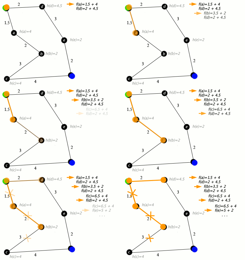
Full worked example: run A* by handFull worked example: হাতে A* চালাই
Edges: S–A = 2, S–B = 3, A–C = 4, B–C = 2, C–G = 4, A–G = 10. Heuristics: h(S)=8, h(A)=7, h(B)=6, h(C)=4, h(G)=0.
Step 1. Open list: {S with f = 0 + 8 = 8}. Expand S.
→ A: g = 2, f = 2 + 7 = 9. → B: g = 3, f = 3 + 6 = 9.
Open: {A(9), B(9)} — a tie; take A (alphabetical).
Step 2. Expand A (f = 9).
→ C via A: g = 2 + 4 = 6, f = 6 + 4 = 10. → G via A: g = 2 + 10 = 12, f = 12 + 0 = 12.
Open: {B(9), C(10), G(12)}. Smallest is B.
Step 3. Expand B (f = 9).
→ C via B: g = 3 + 2 = 5, f = 5 + 4 = 9. This is cheaper than the old C (g = 6), so we update C: parent = B, g = 5.
Open: {C(9), G(12)}. Smallest is C.
Step 4. Expand C (f = 9).
→ G via C: g = 5 + 4 = 9, f = 9 + 0 = 9. Better than the old G(12), so update G: parent = C.
Open: {G(9)}.
Step 5. Expand G — it is the goal. Stop.
Answer: path = S → B → C → G, total cost = 3 + 2 + 4 = 9. Note how A* first tried A but corrected itself using f values. Greedy best-first here would go S → B (h=6) → C (h=4) → G and get lucky, but greedy has no guarantee in general; A* with this admissible h is guaranteed optimal.
Edge: S–A = 2, S–B = 3, A–C = 4, B–C = 2, C–G = 4, A–G = 10। Heuristic: h(S)=8, h(A)=7, h(B)=6, h(C)=4, h(G)=0।
Step 1. Open list: {S, f = 0 + 8 = 8}। S expand করি।
→ A: g = 2, f = 2 + 7 = 9। → B: g = 3, f = 3 + 6 = 9।
Open: {A(9), B(9)} — tie; A নিই (alphabetical)।
Step 2. A expand করি (f = 9)।
→ A দিয়ে C: g = 2 + 4 = 6, f = 6 + 4 = 10। → A দিয়ে G: g = 2 + 10 = 12, f = 12।
Open: {B(9), C(10), G(12)}। সবচেয়ে ছোট B।
Step 3. B expand করি (f = 9)।
→ B দিয়ে C: g = 3 + 2 = 5, f = 5 + 4 = 9। পুরনো C (g = 6)-এর চেয়ে সস্তা, তাই C update করি: parent = B, g = 5।
Open: {C(9), G(12)}। সবচেয়ে ছোট C।
Step 4. C expand করি (f = 9)।
→ C দিয়ে G: g = 5 + 4 = 9, f = 9। পুরনো G(12)-এর চেয়ে ভালো, তাই G update: parent = C।
Open: {G(9)}।
Step 5. G expand করি — এটাই goal। থামি।
Answer: path = S → B → C → G, total cost = 3 + 2 + 4 = 9। খেয়াল করুন, A* প্রথমে A চেষ্টা করেছিল, কিন্তু f value দিয়ে নিজেকে ঠিক করে নিয়েছে। এখানে greedy best-first-ও S → B (h=6) → C (h=4) → G যেত — কপাল ভালো ছিল; কিন্তু general-ভাবে greedy-র কোনো guarantee নেই। Admissible h দিয়ে A*-এর optimal হওয়া guaranteed।
Hill climbing and the local maximum problem
Hill climbing is a local search: from the current state, move to the best neighbor; repeat; stop when no neighbor is better. It uses almost no memory. But it can get stuck:
- Local maximum: a peak that is better than its neighbors but worse than the global best. Hill climbing stops there.
- Plateau: a flat area — no neighbor is better, so the search wanders or halts.
- Ridge: a narrow high path where every single move looks downhill.
Fixes: random restarts (run again from random starts), or simulated annealing (sometimes accept a worse move with a probability that shrinks over time).
Hill climbing আর local maximum problem
Hill climbing একটা local search: current state থেকে সবচেয়ে ভালো neighbor-এ যান; repeat করুন; কোনো neighbor ভালো না হলে থামুন। Memory প্রায় লাগেই না। কিন্তু আটকে যেতে পারে:
- Local maximum: এমন চূড়া, যেটা তার neighbor-দের চেয়ে ভালো কিন্তু global best-এর চেয়ে খারাপ। Hill climbing সেখানেই থেমে যায়।
- Plateau: সমতল জায়গা — কোনো neighbor ভালো না, তাই search ঘুরপাক খায় বা থেমে যায়।
- Ridge: সরু উঁচু path, যেখানে প্রতিটা single move-কে নিচের দিকে মনে হয়।
সমাধান: random restart (random জায়গা থেকে আবার চালানো), বা simulated annealing (মাঝে মাঝে খারাপ move-ও accept করা, সময়ের সাথে সেই probability কমে)।
Probabilistic vs Heuristic Search (Asked 2024!)Probabilistic vs Heuristic Search (2024-এ এসেছিল!)
BUET (April 2024) directly asked the difference between these two families. Learn it as two ideas:
- Heuristic search uses domain knowledge: a heuristic estimate \( h(n) \) of "how close is this node to the goal". The estimate guides a deterministic exploration — run it twice on the same input and you get the same node order. Examples: A*, greedy best-first search, hill climbing.
- Probabilistic (stochastic) search uses randomness as its main tool. It makes random moves, random restarts, or accepts worse states with some probability. The randomness lets it escape local optima and explore parts of the space a greedy climber would never visit. Two runs can give different answers. Examples: simulated annealing, genetic algorithms, random-restart hill climbing, Monte Carlo methods.
They are not enemies — simulated annealing still uses the objective value like a heuristic, but it adds randomness on top so it does not get stuck.
BUET (April 2024) সরাসরি এই দুই family-র পার্থক্য জিজ্ঞেস করেছিল। দুইটা idea হিসেবে শিখুন:
- Heuristic search ব্যবহার করে domain knowledge: একটা heuristic estimate \( h(n) \) — "এই node goal-এর কত কাছে"। এই estimate একটা deterministic exploration-কে guide করে — একই input-এ দুইবার চালালে একই node order পাবেন। Example: A*, greedy best-first search, hill climbing।
- Probabilistic (stochastic) search-এর মূল হাতিয়ার randomness। এটা random move নেয়, random restart করে, বা কিছু probability-তে খারাপ state-ও accept করে। এই randomness-এর কারণে এটা local optima থেকে বের হতে পারে আর space-এর এমন জায়গা explore করে, যেখানে greedy climber কখনো যেত না। দুইবার চালালে আলাদা answer আসতে পারে। Example: simulated annealing, genetic algorithms, random-restart hill climbing, Monte Carlo methods।
এরা শত্রু না — simulated annealing-ও objective value-কে heuristic-এর মতো ব্যবহার করে, কিন্তু আটকে না যাওয়ার জন্য উপরে randomness যোগ করে।
| AspectAspect | Heuristic searchHeuristic search | Probabilistic searchProbabilistic search |
|---|---|---|
| Guidance sourceGuidance-এর উৎস | Domain-knowledge estimate \( h(n) \)Domain-knowledge estimate \( h(n) \) | Randomness (random moves / restarts / mutations)Randomness (random move / restart / mutation) |
| Deterministic?Deterministic? | Yes — same input, same resultYes — একই input, একই result | No — different runs can differNo — আলাদা run-এ আলাদা হতে পারে |
| Optimality guaranteeOptimality guarantee | A* with admissible \( h \): guaranteed optimal; greedy/hill climbing: noneAdmissible \( h \) সহ A*: guaranteed optimal; greedy/hill climbing: নেই | No hard guarantee — usually a good solution with high probability (simulated annealing is optimal only in a slow-cooling limit)শক্ত guarantee নেই — সাধারণত high probability-তে ভালো solution (simulated annealing শুধু খুব ধীরে ঠান্ডা করার limit-এ optimal) |
| Example algorithmsExample algorithm | A*, greedy best-first, hill climbingA*, greedy best-first, hill climbing | Simulated annealing, genetic algorithms, random restarts, Monte CarloSimulated annealing, genetic algorithms, random restarts, Monte Carlo |
| When to useকখন ব্যবহার করবেন | A good \( h \) exists and you need the (optimal) path itselfভালো \( h \) আছে আর আপনার (optimal) path-টাই দরকার | Huge/rugged space, many local optima, no good \( h \) — a "good enough" state is fineবিশাল/এবড়োখেবড়ো space, অনেক local optima, ভালো \( h \) নেই — "যথেষ্ট ভালো" state হলেই চলে |
Minimax for games
In a two-player game (chess, tic-tac-toe), my opponent works against me. Minimax assumes both players play perfectly:
- MAX (me) picks the child with the largest value.
- MIN (opponent) picks the child with the smallest value.
- Leaf values come from a utility/evaluation function. Values flow up the tree.
Game-এর জন্য minimax
দুই player-এর game-এ (chess, tic-tac-toe) opponent আমার বিরুদ্ধে খেলে। Minimax ধরে নেয় দুজনেই perfect খেলে:
- MAX (আমি) সবচেয়ে বড় value-র child নেয়।
- MIN (opponent) সবচেয়ে ছোট value-র child নেয়।
- Leaf-এর value আসে utility/evaluation function থেকে। Value গুলো tree-র উপরের দিকে উঠে যায়।
Root is MAX. It has two MIN children. Leaves: left MIN sees (3, 5); right MIN sees (2, 9).
- Left MIN node: min(3, 5) = 3.
- Right MIN node: min(2, 9) = 2.
- Root MAX: max(3, 2) = 3. So the best move for MAX is the left branch, and the game value is 3.
Alpha-beta pruning idea: after finishing the left MIN (value 3), MAX knows it can get at least 3 (\( \alpha = 3 \)). Exploring the right MIN, the first leaf is 2. Now the right MIN's value will be \( \le 2 \), which is already worse than 3 for MAX. So we skip (prune) leaf 9 — it cannot change the answer. Alpha-beta always gives the same result as minimax but can look at far fewer nodes; with perfect move ordering it examines about \( O(b^{m/2}) \) nodes instead of \( O(b^m) \).
Root হলো MAX। তার দুটো MIN child। Leaf: বাম MIN দেখে (3, 5); ডান MIN দেখে (2, 9)।
- বাম MIN node: min(3, 5) = 3।
- ডান MIN node: min(2, 9) = 2।
- Root MAX: max(3, 2) = 3। তাই MAX-এর best move বাম branch, আর game value হলো 3।
Alpha-beta pruning-এর idea: বাম MIN শেষ করার পরে (value 3) MAX জানে সে অন্তত 3 পাবে (\( \alpha = 3 \))। ডান MIN explore করতে গিয়ে প্রথম leaf 2 পাওয়া গেল। এখন ডান MIN-এর value হবে \( \le 2 \), যা MAX-এর জন্য 3-এর চেয়ে খারাপ। তাই leaf 9 skip (prune) করি — ওটা answer বদলাতে পারবে না। Alpha-beta সবসময় minimax-এর মতোই result দেয়, কিন্তু অনেক কম node দেখে; perfect move ordering হলে \( O(b^m) \)-এর বদলে প্রায় \( O(b^{m/2}) \) node দেখে।
3. Knowledge Representation (KR)3. Knowledge Representation (KR)
An intelligent agent needs to store what it knows and reason with it (derive new facts). Knowledge representation is about how to write knowledge so a computer can use it.
Logic for KR
Propositional logic: the world is described by simple true/false statements (propositions) joined by connectives:
- \( \neg \) (NOT), \( \wedge \) (AND), \( \vee \) (OR), \( \rightarrow \) (implies), \( \leftrightarrow \) (if and only if).
- Example: \( Rain \rightarrow WetRoad \) means "if it rains, the road is wet."
First-order logic (FOL): more powerful. It adds objects, relations, functions, and quantifiers:
- \( \forall \) = "for all", \( \exists \) = "there exists".
- \( \forall x \; Human(x) \rightarrow Mortal(x) \) — "all humans are mortal."
- \( Human(Socrates) \) is a fact. From the rule + fact, we can infer \( Mortal(Socrates) \).
A knowledge base (KB) is a set of such facts (known truths) and rules (if–then statements). An inference engine applies rules to facts to produce new facts. The key inference rule is Modus Ponens: from \( P \) and \( P \rightarrow Q \), conclude \( Q \).
একটা intelligent agent-এর দরকার যা জানে তা store করা আর তা দিয়ে reason করা (নতুন fact বের করা)। Knowledge representation হলো knowledge এমনভাবে লেখা, যাতে computer সেটা ব্যবহার করতে পারে।
KR-এর জন্য logic
Propositional logic: পুরো world-কে simple true/false statement (proposition) দিয়ে বর্ণনা করা হয়, connective দিয়ে জোড়া লাগিয়ে:
- \( \neg \) (NOT), \( \wedge \) (AND), \( \vee \) (OR), \( \rightarrow \) (implies), \( \leftrightarrow \) (if and only if)।
- Example: \( Rain \rightarrow WetRoad \) মানে "বৃষ্টি হলে রাস্তা ভেজা।"
First-order logic (FOL): আরও শক্তিশালী। এতে object, relation, function আর quantifier যোগ হয়:
- \( \forall \) = "সবার জন্য", \( \exists \) = "অন্তত একটা আছে"।
- \( \forall x \; Human(x) \rightarrow Mortal(x) \) — "সব মানুষ মরণশীল।"
- \( Human(Socrates) \) একটা fact। Rule + fact থেকে আমরা infer করতে পারি \( Mortal(Socrates) \)।
Knowledge base (KB) হলো এমন fact (জানা সত্য) আর rule (if–then statement)-এর সেট। Inference engine fact-এর উপর rule apply করে নতুন fact বানায়। মূল inference rule হলো Modus Ponens: \( P \) আর \( P \rightarrow Q \) থেকে \( Q \) conclude করা।
Forward chaining vs backward chaining
- Forward chaining (data-driven): start from known facts. Fire every rule whose conditions are satisfied. Add the new facts. Repeat until the goal appears (or nothing new is produced). "From facts, move forward to conclusions."
- Backward chaining (goal-driven): start from the goal. Ask: which rule can conclude this goal? Then try to prove that rule's conditions as sub-goals. Recurse down to known facts. "From the goal, move backward to facts." Prolog works this way.
Forward chaining vs backward chaining
- Forward chaining (data-driven): জানা fact থেকে শুরু। যে rule-এর condition মিলে যায়, সেটা fire করি। নতুন fact যোগ করি। Goal না আসা পর্যন্ত (বা নতুন কিছু না আসা পর্যন্ত) repeat। "Fact থেকে সামনে এগিয়ে conclusion-এ।"
- Backward chaining (goal-driven): goal থেকে শুরু। প্রশ্ন করি: কোন rule এই goal conclude করতে পারে? তারপর সেই rule-এর condition গুলোকে sub-goal হিসেবে প্রমাণ করার চেষ্টা করি। জানা fact পর্যন্ত recurse করি। "Goal থেকে পেছনে গিয়ে fact-এ।" Prolog এভাবেই কাজ করে।
Knowledge base:
- R1: \( A \wedge B \rightarrow C \)
- R2: \( C \rightarrow D \)
- R3: \( D \wedge E \rightarrow F \)
- Facts: \( A, B, E \). Goal: prove \( F \).
Forward chaining:
- Facts = {A, B, E}. R1 needs A and B — both known → fire R1, add C.
- Facts = {A, B, E, C}. R2 needs C → fire R2, add D.
- Facts = {A, B, E, C, D}. R3 needs D and E — both known → fire R3, add F. Goal reached. ✔
Backward chaining:
- Goal F. R3 concludes F, so prove sub-goals D and E.
- E is a fact ✔. For D: R2 concludes D, so prove C.
- For C: R1 concludes C, so prove A and B — both facts ✔. So C ✔, then D ✔, then F ✔.
Same answer, opposite directions. Forward chaining may derive extra facts you never needed; backward chaining only touches rules related to the goal.
Knowledge base:
- R1: \( A \wedge B \rightarrow C \)
- R2: \( C \rightarrow D \)
- R3: \( D \wedge E \rightarrow F \)
- Fact: \( A, B, E \)। Goal: \( F \) প্রমাণ করা।
Forward chaining:
- Fact = {A, B, E}। R1-এর দরকার A আর B — দুটোই জানা → R1 fire, C যোগ হলো।
- Fact = {A, B, E, C}। R2-এর দরকার C → R2 fire, D যোগ হলো।
- Fact = {A, B, E, C, D}। R3-এর দরকার D আর E — দুটোই জানা → R3 fire, F যোগ হলো। Goal পাওয়া গেল। ✔
Backward chaining:
- Goal F। R3 F conclude করে, তাই sub-goal D আর E প্রমাণ করতে হবে।
- E একটা fact ✔। D-এর জন্য: R2 D conclude করে, তাই C প্রমাণ করতে হবে।
- C-এর জন্য: R1 C conclude করে, তাই A আর B প্রমাণ করতে হবে — দুটোই fact ✔। তাহলে C ✔, তারপর D ✔, তারপর F ✔।
Answer একই, দিক উল্টো। Forward chaining দরকার নেই এমন বাড়তি fact-ও বানাতে পারে; backward chaining শুধু goal-এর সাথে জড়িত rule গুলোই ধরে।
Other KR methods
- Semantic network: a graph of concepts. Nodes = objects/concepts, labeled edges = relations. Common links:
is-a(Sparrow is-a Bird),has-a(Bird has-a Wings). Properties can be inherited down is-a links: Sparrow inherits "can fly" from Bird. - Frames: a record-like structure for one concept, with slots (attributes) and fillers (values or defaults). Example: frame
Birdwith slotslegs: 2,flies: yes. Frames are basically the ancestor of objects/classes in OOP. - Ontology: a formal, agreed vocabulary of the concepts in a domain and the relations between them (a shared "map of meaning").
Rule-based expert systems
An expert system tries to act like a human expert in a narrow field (medical diagnosis, machine troubleshooting). Its parts:
- Knowledge base: if–then rules collected from experts.
- Inference engine: applies rules (forward or backward chaining).
- Working memory: the current known facts of a session.
- User interface and an explanation facility ("why did you conclude this?").
Famous classic example: MYCIN, which suggested antibiotics for blood infections using about 600 rules.
অন্যান্য KR method
- Semantic network: concept-এর একটা graph। Node = object/concept, labeled edge = relation। Common link:
is-a(Sparrow is-a Bird),has-a(Bird has-a Wings)। is-a link ধরে property inherit হয়: Sparrow, Bird থেকে "can fly" inherit করে। - Frames: একটা concept-এর জন্য record-এর মতো structure, যাতে থাকে slot (attribute) আর filler (value বা default)। Example:
Birdframe, slotlegs: 2,flies: yes। Frames আসলে OOP-এর object/class-এর পূর্বপুরুষ। - Ontology: একটা domain-এর concept আর তাদের মধ্যের relation-এর formal, সবার-মানা vocabulary (একটা shared "অর্থের map")।
Rule-based expert system
Expert system একটা ছোট field-এ human expert-এর মতো কাজ করার চেষ্টা করে (medical diagnosis, machine troubleshooting)। এর অংশগুলো:
- Knowledge base: expert-দের কাছ থেকে নেওয়া if–then rule।
- Inference engine: rule apply করে (forward বা backward chaining)।
- Working memory: একটা session-এর current জানা fact।
- User interface আর explanation facility ("কেন এই conclusion দিলে?")।
বিখ্যাত classic example: MYCIN — প্রায় ৬০০টা rule দিয়ে রক্তের infection-এর জন্য antibiotic suggest করত।
4. Basic Machine Learning Concepts4. Basic Machine Learning Concepts
Machine Learning (ML) means: instead of writing rules by hand, we show the computer data and let it learn patterns from the data. AI, ML, and Deep Learning fit inside each other:
- AI: the big field — making machines act intelligently (search, logic, planning, learning, everything).
- ML: a part of AI — systems that improve from data/experience.
- Deep Learning (DL): a part of ML — learning with many-layered neural networks.
Machine Learning (ML) মানে: হাতে rule না লিখে computer-কে data দেখাই, আর data থেকে সে pattern শেখে। AI, ML আর Deep Learning একটার ভেতরে আরেকটা:
- AI: বড় field — machine-কে intelligent-ভাবে কাজ করানো (search, logic, planning, learning, সব কিছু)।
- ML: AI-এর একটা অংশ — যে system data/experience থেকে ভালো হয়।
- Deep Learning (DL): ML-এর একটা অংশ — অনেক layer-এর neural network দিয়ে শেখা।
Three types of learningতিন ধরনের learning
| TypeType | Data givenযে data দেওয়া হয় | GoalGoal | ExamplesExample |
|---|---|---|---|
| Supervised | Inputs with correct answers (labels)Input সহ সঠিক উত্তর (label) | Predict the label for new inputsনতুন input-এর label predict করা | Spam detection, house price prediction, disease diagnosisSpam detection, house price prediction, disease diagnosis |
| Unsupervised | Inputs only, no labelsশুধু input, কোনো label নেই | Find hidden structure/groupsলুকানো structure/group খুঁজে বের করা | Customer segmentation (clustering), dimensionality reduction (PCA)Customer segmentation (clustering), dimensionality reduction (PCA) |
| Reinforcement | No dataset; an agent acts and gets rewards/penaltiesDataset নেই; agent কাজ করে আর reward/penalty পায় | Learn a policy that maximizes total rewardএমন policy শেখা, যা total reward maximize করে | Game playing (chess, Go), robot controlGame খেলা (chess, Go), robot control |
Dataset words you must know
- Feature: one input property of an example (age, size, pixel value). A row's features form the input vector \( x \).
- Label (target): the correct answer \( y \) for that example (e.g., "spam" / "not spam", or a price).
- Training set: data used to fit the model (commonly ~60–80%).
- Validation set: data used to tune choices (hyperparameters, which model). The model does not train on it.
- Test set: kept locked until the very end; used once to report the final honest performance.
Overfitting vs underfitting
- Underfitting: the model is too simple. It does badly on training data and new data. (High bias.)
- Overfitting: the model is too complex. It memorizes the training data — great training accuracy, bad accuracy on new (test) data. (High variance.)
- Good fit: in between — learns the true pattern, ignores the noise.
Dataset-এর যে শব্দগুলো জানতেই হবে
- Feature: একটা example-এর একটা input property (age, size, pixel value)। এক row-এর feature গুলো মিলে input vector \( x \)।
- Label (target): সেই example-এর সঠিক উত্তর \( y \) (যেমন "spam" / "not spam", বা একটা price)।
- Training set: model fit করার data (সাধারণত ~৬০–৮০%)।
- Validation set: choice tune করার data (hyperparameter, কোন model)। Model এটার উপর train হয় না।
- Test set: একদম শেষ পর্যন্ত তালাবদ্ধ; final সৎ performance report করতে একবারই ব্যবহার হয়।
Overfitting vs underfitting
- Underfitting: model বেশি simple। Training data-তেও খারাপ, নতুন data-তেও খারাপ। (High bias।)
- Overfitting: model বেশি complex। Training data মুখস্থ করে ফেলে — training accuracy দারুণ, কিন্তু নতুন (test) data-তে খারাপ। (High variance।)
- Good fit: মাঝামাঝি — আসল pattern শেখে, noise ignore করে।

Bias–variance idea
Prediction error has two main parts:
- Bias: error from wrong assumptions — the model is too simple to capture the truth. High bias → underfitting.
- Variance: error from being too sensitive to the particular training sample — the model changes a lot if the data changes slightly. High variance → overfitting.
There is a trade-off: making a model more complex lowers bias but raises variance. We want the sweet spot in the middle.
Cross-validation
k-fold cross-validation: split the data into \( k \) equal folds (say \( k = 5 \)). Train on \( k-1 \) folds, test on the remaining fold. Repeat \( k \) times so every fold is the test fold once. Average the \( k \) scores. This gives a more reliable estimate than one single split, especially with small datasets.
Bias–variance-এর idea
Prediction error-এর দুটো প্রধান অংশ:
- Bias: ভুল assumption থেকে আসা error — model এত simple যে আসল সত্যটা ধরতে পারে না। High bias → underfitting।
- Variance: নির্দিষ্ট training sample-এর প্রতি অতি সংবেদনশীল হওয়ার error — data একটু বদলালেই model অনেক বদলে যায়। High variance → overfitting।
এখানে একটা trade-off আছে: model complex করলে bias কমে কিন্তু variance বাড়ে। আমরা চাই মাঝের sweet spot।
Cross-validation
k-fold cross-validation: data-কে \( k \)-টা সমান fold-এ ভাগ করুন (ধরুন \( k = 5 \))। \( k-1 \)-টা fold-এ train করুন, বাকি fold-এ test করুন। \( k \) বার repeat করুন, যাতে প্রতিটা fold একবার test fold হয়। \( k \)-টা score-এর average নিন। একবারের single split-এর চেয়ে এটা বেশি নির্ভরযোগ্য estimate দেয়, বিশেষ করে ছোট dataset-এ।
Evaluation metrics: confusion matrix & friendsEvaluation metrics: confusion matrix আর তার বন্ধুরা
For a two-class problem (Positive / Negative), the confusion matrix counts four outcomes:
- TP (True Positive): actually positive, predicted positive. ✔
- TN (True Negative): actually negative, predicted negative. ✔
- FP (False Positive): actually negative, but predicted positive. ("false alarm", Type I error)
- FN (False Negative): actually positive, but predicted negative. ("missed case", Type II error)
দুই-class problem-এ (Positive / Negative), confusion matrix চারটা outcome গোনে:
- TP (True Positive): আসলে positive, predict-ও positive। ✔
- TN (True Negative): আসলে negative, predict-ও negative। ✔
- FP (False Positive): আসলে negative, কিন্তু predict positive। ("false alarm", Type I error)
- FN (False Negative): আসলে positive, কিন্তু predict negative। ("miss হওয়া case", Type II error)
| Predicted Positive | Predicted Negative | |
|---|---|---|
| Actual Positive | TP = 40 | FN = 10 |
| Actual Negative | FP = 20 | TN = 30 |
Step 1 — Accuracy: \( (40 + 30) / 100 = 70/100 = \mathbf{0.70} \) → 70% of all predictions are correct.
Step 2 — Precision: \( 40 / (40 + 20) = 40/60 \approx \mathbf{0.667} \) → of everyone the model called "sick", 66.7% really are sick.
Step 3 — Recall: \( 40 / (40 + 10) = 40/50 = \mathbf{0.80} \) → of all truly sick patients, the model caught 80%.
Step 4 — F1 score:
\[ F1 = \frac{2 \times 0.667 \times 0.80}{0.667 + 0.80} = \frac{1.067}{1.467} \approx \mathbf{0.727} \]F1 is the harmonic mean of precision and recall — it is high only when both are high.
| Predicted Positive | Predicted Negative | |
|---|---|---|
| Actual Positive | TP = 40 | FN = 10 |
| Actual Negative | FP = 20 | TN = 30 |
Step 1 — Accuracy: \( (40 + 30) / 100 = 70/100 = \mathbf{0.70} \) → সব prediction-এর ৭০% সঠিক।
Step 2 — Precision: \( 40 / (40 + 20) = 40/60 \approx \mathbf{0.667} \) → model যাদের "sick" বলেছে, তাদের ৬৬.৭% সত্যিই sick।
Step 3 — Recall: \( 40 / (40 + 10) = 40/50 = \mathbf{0.80} \) → সত্যিকারের sick patient-দের ৮০% model ধরতে পেরেছে।
Step 4 — F1 score:
\[ F1 = \frac{2 \times 0.667 \times 0.80}{0.667 + 0.80} = \frac{1.067}{1.467} \approx \mathbf{0.727} \]F1 হলো precision আর recall-এর harmonic mean — দুটোই high হলে তবেই F1 high হয়।
5. Classification and Regression5. Classification and Regression
Both are supervised learning. The difference is the type of output:
- Regression: predict a continuous number (house price, temperature).
- Classification: predict a category (spam / not spam, digit 0–9).
Linear regression
We assume the output is roughly a straight-line function of the input:
দুটোই supervised learning। পার্থক্য output-এর ধরনে:
- Regression: একটা continuous number predict করা (house price, temperature)।
- Classification: একটা category predict করা (spam / not spam, digit 0–9)।
Linear regression
আমরা ধরে নিই output মোটামুটি input-এর একটা সরলরেখা-ধরনের function:
Training = finding the \( w, b \) that make the Mean Squared Error smallest. The closed-form least squares answer:
Training = সেই \( w, b \) খুঁজে বের করা, যা Mean Squared Error সবচেয়ে ছোট করে। Closed-form least squares answer:
Data: hours studied \( x \) vs marks \( y \): (1, 2), (2, 3), (3, 5), (4, 6).
Step 1 — means: \( \bar{x} = (1+2+3+4)/4 = 2.5 \), \( \bar{y} = (2+3+5+6)/4 = 4 \).
Step 2 — numerator \( \sum (x_i-\bar{x})(y_i-\bar{y}) \):
- \( (1-2.5)(2-4) = (-1.5)(-2) = 3 \)
- \( (2-2.5)(3-4) = (-0.5)(-1) = 0.5 \)
- \( (3-2.5)(5-4) = (0.5)(1) = 0.5 \)
- \( (4-2.5)(6-4) = (1.5)(2) = 3 \)
Sum = \( 3 + 0.5 + 0.5 + 3 = 7 \).
Step 3 — denominator \( \sum (x_i-\bar{x})^2 = 2.25 + 0.25 + 0.25 + 2.25 = 5 \).
Step 4 — slope and intercept: \( w = 7/5 = \mathbf{1.4} \); \( b = 4 - 1.4 \times 2.5 = 4 - 3.5 = \mathbf{0.5} \).
Answer: \( \hat{y} = 1.4x + 0.5 \). Prediction for \( x = 5 \) hours: \( 1.4 \times 5 + 0.5 = 7.5 \) marks.
Data: পড়ার ঘণ্টা \( x \) vs marks \( y \): (1, 2), (2, 3), (3, 5), (4, 6)।
Step 1 — mean: \( \bar{x} = (1+2+3+4)/4 = 2.5 \), \( \bar{y} = (2+3+5+6)/4 = 4 \)।
Step 2 — লব \( \sum (x_i-\bar{x})(y_i-\bar{y}) \):
- \( (1-2.5)(2-4) = (-1.5)(-2) = 3 \)
- \( (2-2.5)(3-4) = (-0.5)(-1) = 0.5 \)
- \( (3-2.5)(5-4) = (0.5)(1) = 0.5 \)
- \( (4-2.5)(6-4) = (1.5)(2) = 3 \)
যোগফল = \( 3 + 0.5 + 0.5 + 3 = 7 \)।
Step 3 — হর \( \sum (x_i-\bar{x})^2 = 2.25 + 0.25 + 0.25 + 2.25 = 5 \)।
Step 4 — slope আর intercept: \( w = 7/5 = \mathbf{1.4} \); \( b = 4 - 1.4 \times 2.5 = 4 - 3.5 = \mathbf{0.5} \)।
Answer: \( \hat{y} = 1.4x + 0.5 \)। \( x = 5 \) ঘণ্টার prediction: \( 1.4 \times 5 + 0.5 = 7.5 \) marks।
Logistic regression + sigmoid
Despite the name, logistic regression is a classification method. It computes \( z = wx + b \), then squashes \( z \) into a probability between 0 and 1 using the sigmoid function:
Logistic regression + sigmoid
নাম শুনে যা-ই মনে হোক, logistic regression আসলে একটা classification method। এটা \( z = wx + b \) হিসাব করে, তারপর sigmoid function দিয়ে \( z \)-কে 0 থেকে 1-এর মধ্যে একটা probability-তে চেপে দেয়:
If \( \sigma(z) \ge 0.5 \) (i.e. \( z \ge 0 \)) predict class 1; otherwise class 0. Note \( \sigma(0) = 0.5 \).
\( \sigma(z) \ge 0.5 \) হলে (মানে \( z \ge 0 \)) class 1 predict করি; নাহলে class 0। মনে রাখুন \( \sigma(0) = 0.5 \)।

K-Nearest Neighbors (KNN)
KNN is a lazy, simple classifier: to classify a new point, find the \( K \) closest training points (usually Euclidean distance) and take a majority vote of their classes. No real "training" happens — the data itself is the model. Choose odd \( K \) to avoid ties.
K-Nearest Neighbors (KNN)
KNN একটা lazy, simple classifier: নতুন point classify করতে training data-র সবচেয়ে কাছের \( K \)-টা point খুঁজুন (সাধারণত Euclidean distance), তারপর তাদের class-এর majority vote নিন। আসল "training" কিছু হয় না — data-ই model। Tie এড়াতে বিজোড় \( K \) নিন।
Training data: P1(2, 3, class +), P2(4, 4, class +), P3(4, 2, class −), P4(6, 6, class −), P5(1, 1, class −).
Step 1 — distances to (3, 3):
- P1: \( \sqrt{(3-2)^2 + (3-3)^2} = \sqrt{1} = 1.00 \)
- P2: \( \sqrt{(3-4)^2 + (3-4)^2} = \sqrt{2} \approx 1.41 \)
- P3: \( \sqrt{(3-4)^2 + (3-2)^2} = \sqrt{2} \approx 1.41 \)
- P4: \( \sqrt{9 + 9} = \sqrt{18} \approx 4.24 \)
- P5: \( \sqrt{4 + 4} = \sqrt{8} \approx 2.83 \)
Step 2 — pick the 3 nearest: P1 (+), P2 (+), P3 (−).
Step 3 — majority vote: two "+" vs one "−" → predict class +.
Note: with K = 1 the answer would come only from P1 (+). With very large K, faraway points start voting and the boundary gets too smooth — K controls the bias–variance trade-off.
Training data: P1(2, 3, class +), P2(4, 4, class +), P3(4, 2, class −), P4(6, 6, class −), P5(1, 1, class −)।
Step 1 — (3, 3) থেকে distance:
- P1: \( \sqrt{(3-2)^2 + (3-3)^2} = \sqrt{1} = 1.00 \)
- P2: \( \sqrt{(3-4)^2 + (3-4)^2} = \sqrt{2} \approx 1.41 \)
- P3: \( \sqrt{(3-4)^2 + (3-2)^2} = \sqrt{2} \approx 1.41 \)
- P4: \( \sqrt{9 + 9} = \sqrt{18} \approx 4.24 \)
- P5: \( \sqrt{4 + 4} = \sqrt{8} \approx 2.83 \)
Step 2 — সবচেয়ে কাছের ৩টা: P1 (+), P2 (+), P3 (−)।
Step 3 — majority vote: দুইটা "+" vs একটা "−" → predict class +।
Note: K = 1 হলে উত্তর আসত শুধু P1 (+) থেকে। K খুব বড় হলে দূরের point-ও vote দেয়, boundary বেশি smooth হয়ে যায় — K-ই bias–variance trade-off control করে।
Decision trees: entropy & information gain
A decision tree asks feature questions ("Is Wind = Strong?") and splits the data at each node. Which feature to split on first? The one with the highest information gain. First we need entropy — a measure of impurity/uncertainty of a set \( S \):
Decision tree: entropy আর information gain
Decision tree feature নিয়ে প্রশ্ন করে ("Wind = Strong কি?") আর প্রতি node-এ data ভাগ করে। প্রথমে কোন feature-এ split করব? যেটার information gain সবচেয়ে বেশি। তার আগে চাই entropy — একটা set \( S \)-এর impurity/uncertainty-র মাপ:
Dataset: 10 samples about playing football — 6 "Yes", 4 "No". Candidate feature: Wind ∈ {Weak, Strong}. Weak has 6 samples (5 Yes, 1 No); Strong has 4 samples (1 Yes, 3 No).
Step 1 — parent entropy:
\[ H(S) = -0.6 \log_2 0.6 - 0.4 \log_2 0.4 = 0.442 + 0.529 = \mathbf{0.971} \]Step 2 — entropy of each branch:
\[ H(\text{Weak}) = -\tfrac{5}{6}\log_2\tfrac{5}{6} - \tfrac{1}{6}\log_2\tfrac{1}{6} = 0.219 + 0.431 = \mathbf{0.650} \] \[ H(\text{Strong}) = -\tfrac{1}{4}\log_2\tfrac{1}{4} - \tfrac{3}{4}\log_2\tfrac{3}{4} = 0.5 + 0.311 = \mathbf{0.811} \]Step 3 — weighted average of children:
\[ \tfrac{6}{10}(0.650) + \tfrac{4}{10}(0.811) = 0.390 + 0.324 = 0.714 \]Step 4 — information gain:
\[ IG(S, \text{Wind}) = 0.971 - 0.714 = \mathbf{0.257} \]Compute IG the same way for every candidate feature; split on the feature with the largest IG. (This is the ID3 algorithm. C4.5 and CART are its famous successors.)
Dataset: football খেলা নিয়ে ১০টা sample — ৬টা "Yes", ৪টা "No"। Candidate feature: Wind ∈ {Weak, Strong}। Weak-এ ৬টা sample (5 Yes, 1 No); Strong-এ ৪টা (1 Yes, 3 No)।
Step 1 — parent entropy:
\[ H(S) = -0.6 \log_2 0.6 - 0.4 \log_2 0.4 = 0.442 + 0.529 = \mathbf{0.971} \]Step 2 — প্রতি branch-এর entropy:
\[ H(\text{Weak}) = -\tfrac{5}{6}\log_2\tfrac{5}{6} - \tfrac{1}{6}\log_2\tfrac{1}{6} = 0.219 + 0.431 = \mathbf{0.650} \] \[ H(\text{Strong}) = -\tfrac{1}{4}\log_2\tfrac{1}{4} - \tfrac{3}{4}\log_2\tfrac{3}{4} = 0.5 + 0.311 = \mathbf{0.811} \]Step 3 — child-দের weighted average:
\[ \tfrac{6}{10}(0.650) + \tfrac{4}{10}(0.811) = 0.390 + 0.324 = 0.714 \]Step 4 — information gain:
\[ IG(S, \text{Wind}) = 0.971 - 0.714 = \mathbf{0.257} \]প্রতিটা candidate feature-এর জন্য একইভাবে IG হিসাব করুন; সবচেয়ে বড় IG-এর feature-এ split করুন। (এটাই ID3 algorithm। C4.5 আর CART এর বিখ্যাত উত্তরসূরি।)
- Simple and easy to understand — the whole algorithm is just "pick the highest-IG feature, split, repeat".
- Interpretable output: the tree reads as human-friendly if–then rules, so you can explain every prediction.
- Handles categorical data naturally (Wind = Weak/Strong) — no distance measure or scaling needed.
- Fast: a greedy pass over features at each node; building and prediction are both quick.
- Picks the most informative attributes first using information gain, so the important features sit near the root and the tree stays short.
- Simple আর বোঝা সহজ — পুরো algorithm-টাই হলো "সবচেয়ে বেশি IG-এর feature নিন, split করুন, repeat করুন"।
- Interpretable output: tree-টা মানুষ-বোধ্য if–then rule-এর মতো পড়া যায়, তাই প্রতিটা prediction ব্যাখ্যা করা যায়।
- Categorical data সরাসরি handle করে (Wind = Weak/Strong) — কোনো distance measure বা scaling লাগে না।
- Fast: প্রতি node-এ feature-গুলোর উপর একটা greedy pass; tree বানানো আর prediction দুটোই দ্রুত।
- Information gain দিয়ে সবচেয়ে informative attribute-গুলো আগে বেছে নেয়, তাই গুরুত্বপূর্ণ feature গুলো root-এর কাছে থাকে আর tree ছোট থাকে।
Naive Bayes
Naive Bayes uses Bayes' theorem with one big ("naive") assumption: features are independent given the class.
Naive Bayes
Naive Bayes Bayes' theorem ব্যবহার করে, একটা বড় ("naive") assumption সহ: class জানা থাকলে feature-গুলো independent।
Out of 10 emails, 4 are spam and 6 are not (ham). The word "free" appears in 3 of the 4 spam emails and in 1 of the 6 ham emails. A new email contains "free". Spam or ham?
Step 1 — priors: \( P(\text{spam}) = 0.4 \), \( P(\text{ham}) = 0.6 \).
Step 2 — likelihoods: \( P(\text{free} \mid \text{spam}) = 3/4 = 0.75 \); \( P(\text{free} \mid \text{ham}) = 1/6 \approx 0.167 \).
Step 3 — unnormalized posteriors:
- spam: \( 0.75 \times 0.4 = 0.30 \)
- ham: \( 0.167 \times 0.6 = 0.10 \)
Step 4 — normalize: \( P(\text{spam} \mid \text{free}) = 0.30 / (0.30 + 0.10) = \mathbf{0.75} \). Predict spam.
With many words, just multiply all the \( P(x_i \mid C) \) terms. If a word never appeared in a class, its probability is 0 and kills the product — fix with Laplace smoothing (add 1 to every count).
১০টা email-এর মধ্যে ৪টা spam, ৬টা ham। "free" শব্দটা ৪টা spam-এর ৩টাতে আছে, আর ৬টা ham-এর ১টাতে। নতুন একটা email-এ "free" আছে। Spam না ham?
Step 1 — prior: \( P(\text{spam}) = 0.4 \), \( P(\text{ham}) = 0.6 \)।
Step 2 — likelihood: \( P(\text{free} \mid \text{spam}) = 3/4 = 0.75 \); \( P(\text{free} \mid \text{ham}) = 1/6 \approx 0.167 \)।
Step 3 — unnormalized posterior:
- spam: \( 0.75 \times 0.4 = 0.30 \)
- ham: \( 0.167 \times 0.6 = 0.10 \)
Step 4 — normalize: \( P(\text{spam} \mid \text{free}) = 0.30 / (0.30 + 0.10) = \mathbf{0.75} \)। Predict: spam।
অনেক শব্দ থাকলে সব \( P(x_i \mid C) \) গুণ করলেই হয়। কোনো শব্দ কোনো class-এ কখনো না এলে তার probability 0 হয়ে পুরো গুণফল মেরে ফেলে — সমাধান Laplace smoothing (প্রতি count-এ 1 যোগ)।
SVM idea: margin and hyperplane
A Support Vector Machine separates two classes with a hyperplane (a line in 2D, a plane in 3D). Among all separating lines, SVM picks the one with the maximum margin — the widest gap between the line and the nearest points of each class. Those nearest points are the support vectors; only they decide the boundary. For data that is not linearly separable, the kernel trick maps points to a higher dimension where a line can separate them.
Perceptron and neural network basics
A perceptron is the simplest artificial neuron:
- Multiply each input by a weight: \( z = w_1 x_1 + w_2 x_2 + \dots + b \).
- Pass \( z \) through an activation function (step, sigmoid, or ReLU \( = \max(0, z) \)).
- Output the result.
A single perceptron can only learn linearly separable functions — famously, it cannot learn XOR. Stacking neurons in layers (input → hidden → output) gives a neural network, which can learn XOR and much more. Training uses backpropagation: compute the output error, send it backwards through the layers using the chain rule, and adjust every weight a little in the direction that reduces the error (gradient descent): \( w \leftarrow w - \eta \frac{\partial E}{\partial w} \), where \( \eta \) is the learning rate.
SVM-এর idea: margin আর hyperplane
Support Vector Machine দুই class-কে একটা hyperplane দিয়ে আলাদা করে (2D-তে line, 3D-তে plane)। সব separating line-এর মধ্যে SVM বেছে নেয় maximum margin-এরটা — line আর দুই class-এর সবচেয়ে কাছের point-গুলোর মাঝের সবচেয়ে চওড়া ফাঁক। সেই কাছের point-গুলোই support vector; শুধু ওরাই boundary ঠিক করে। Data linearly separable না হলে kernel trick point-গুলোকে উঁচু dimension-এ নিয়ে যায়, যেখানে line দিয়ে আলাদা করা যায়।
Perceptron আর neural network-এর basics
Perceptron হলো সবচেয়ে simple artificial neuron:
- প্রতিটা input-কে একটা weight দিয়ে গুণ করা: \( z = w_1 x_1 + w_2 x_2 + \dots + b \)।
- \( z \)-কে একটা activation function-এর ভেতর দিয়ে পাঠানো (step, sigmoid, বা ReLU \( = \max(0, z) \))।
- Result output করা।
একটা single perceptron শুধু linearly separable function শিখতে পারে — বিখ্যাত ঘটনা: এটা XOR শিখতে পারে না। Neuron-গুলোকে layer-এ সাজালে (input → hidden → output) পাওয়া যায় neural network, যেটা XOR-সহ আরও অনেক কিছু শিখতে পারে। Training হয় backpropagation দিয়ে: output-এর error হিসাব করা, chain rule দিয়ে সেটা layer-গুলোর ভেতর দিয়ে পেছনে পাঠানো, আর প্রতিটা weight-কে error কমার দিকে একটু করে বদলানো (gradient descent): \( w \leftarrow w - \eta \frac{\partial E}{\partial w} \), যেখানে \( \eta \) হলো learning rate।
6. Clustering6. Clustering
Quick recap: supervised learning has labels; unsupervised learning does not. Clustering is the main unsupervised task: group similar points together without being told any classes. The algorithm invents the groups itself.
K-means clustering
K-means groups \( n \) points into \( K \) clusters. Steps:
- Choose K and pick \( K \) initial centroids (cluster centers), often random points.
- Assignment step: assign every point to its nearest centroid (Euclidean distance).
- Update step: move each centroid to the mean of the points assigned to it.
- Repeat steps 2–3 until assignments stop changing (convergence).
K-means minimizes the total within-cluster squared distance: \( \sum_k \sum_{x \in C_k} \lVert x - \mu_k \rVert^2 \). It always converges, but possibly to a local optimum — so people run it several times with different starts.
ছোট recap: supervised learning-এ label থাকে; unsupervised-এ থাকে না। Clustering হলো প্রধান unsupervised কাজ: কোনো class না বলে দিয়েই similar point-গুলোকে একসাথে group করা। Algorithm নিজেই group বানায়।
K-means clustering
K-means \( n \)-টা point-কে \( K \)-টা cluster-এ ভাগ করে। Steps:
- K বেছে নিন আর \( K \)-টা initial centroid (cluster center) নিন, প্রায়ই random point।
- Assignment step: প্রতিটা point-কে তার সবচেয়ে কাছের centroid-এ assign করুন (Euclidean distance)।
- Update step: প্রতিটা centroid-কে তার assign হওয়া point-গুলোর mean-এ সরান।
- Assignment বদলানো বন্ধ না হওয়া পর্যন্ত step 2–3 repeat করুন (convergence)।
K-means total within-cluster squared distance minimize করে: \( \sum_k \sum_{x \in C_k} \lVert x - \mu_k \rVert^2 \)। এটা সবসময় converge করে, কিন্তু হয়তো local optimum-এ — তাই আলাদা আলাদা start দিয়ে কয়েকবার চালানো হয়।
Points: P1(1, 1), P2(2, 1), P3(3, 3), P4(5, 4), P5(6, 5). Let K = 2, initial centroids C1 = (1, 1) and C2 = (2, 1).
Iteration 1 — assignment (distance to C1; distance to C2):
- P1(1,1): 0 vs 1 → C1
- P2(2,1): 1 vs 0 → C2
- P3(3,3): \( \sqrt{4+4} = 2.83 \) vs \( \sqrt{1+4} = 2.24 \) → C2
- P4(5,4): \( \sqrt{16+9} = 5.00 \) vs \( \sqrt{9+9} = 4.24 \) → C2
- P5(6,5): \( \sqrt{25+16} = 6.40 \) vs \( \sqrt{16+16} = 5.66 \) → C2
Iteration 1 — update: C1 = mean{P1} = (1, 1). C2 = mean{P2, P3, P4, P5} = \( \left(\frac{2+3+5+6}{4}, \frac{1+3+4+5}{4}\right) = (4, 3.25) \).
Iteration 2 — assignment with C1 = (1,1), C2 = (4, 3.25):
- P1(1,1): 0 vs \( \sqrt{9+5.06} = 3.75 \) → C1
- P2(2,1): 1 vs \( \sqrt{4+5.06} = 3.01 \) → C1 (it switched clusters!)
- P3(3,3): 2.83 vs \( \sqrt{1+0.06} = 1.03 \) → C2
- P4(5,4): 5.00 vs \( \sqrt{1+0.56} = 1.25 \) → C2
- P5(6,5): 6.40 vs \( \sqrt{4+3.06} = 2.66 \) → C2
Iteration 2 — update: C1 = mean{P1, P2} = (1.5, 1). C2 = mean{P3, P4, P5} = \( \left(\frac{3+5+6}{3}, \frac{3+4+5}{3}\right) \approx (4.67, 4) \).
A third assignment pass gives the same clusters {P1, P2} and {P3, P4, P5} → converged. Final answer: clusters {P1, P2} and {P3, P4, P5} with centroids (1.5, 1) and (4.67, 4).
Point: P1(1, 1), P2(2, 1), P3(3, 3), P4(5, 4), P5(6, 5)। ধরি K = 2, initial centroid C1 = (1, 1) আর C2 = (2, 1)।
Iteration 1 — assignment (C1-এর distance; C2-এর distance):
- P1(1,1): 0 vs 1 → C1
- P2(2,1): 1 vs 0 → C2
- P3(3,3): \( \sqrt{4+4} = 2.83 \) vs \( \sqrt{1+4} = 2.24 \) → C2
- P4(5,4): \( \sqrt{16+9} = 5.00 \) vs \( \sqrt{9+9} = 4.24 \) → C2
- P5(6,5): \( \sqrt{25+16} = 6.40 \) vs \( \sqrt{16+16} = 5.66 \) → C2
Iteration 1 — update: C1 = mean{P1} = (1, 1)। C2 = mean{P2, P3, P4, P5} = \( \left(\frac{2+3+5+6}{4}, \frac{1+3+4+5}{4}\right) = (4, 3.25) \)।
Iteration 2 — assignment, C1 = (1,1), C2 = (4, 3.25) দিয়ে:
- P1(1,1): 0 vs \( \sqrt{9+5.06} = 3.75 \) → C1
- P2(2,1): 1 vs \( \sqrt{4+5.06} = 3.01 \) → C1 (cluster বদলে গেল!)
- P3(3,3): 2.83 vs \( \sqrt{1+0.06} = 1.03 \) → C2
- P4(5,4): 5.00 vs \( \sqrt{1+0.56} = 1.25 \) → C2
- P5(6,5): 6.40 vs \( \sqrt{4+3.06} = 2.66 \) → C2
Iteration 2 — update: C1 = mean{P1, P2} = (1.5, 1)। C2 = mean{P3, P4, P5} = \( \left(\frac{3+5+6}{3}, \frac{3+4+5}{3}\right) \approx (4.67, 4) \)।
তৃতীয়বার assignment করলে একই cluster {P1, P2} আর {P3, P4, P5} পাওয়া যায় → converged। Final answer: cluster {P1, P2} আর {P3, P4, P5}, centroid (1.5, 1) আর (4.67, 4)।
Choosing K: the elbow method
Run K-means for K = 1, 2, 3, ... and plot the total within-cluster squared distance (WCSS/inertia) against K. The curve always goes down, but at some K it stops dropping fast and bends like an elbow. Pick that K — after the elbow, extra clusters buy little improvement.
Hierarchical clustering & dendrogram
Agglomerative (bottom-up) hierarchical clustering: start with every point as its own cluster; repeatedly merge the two closest clusters; stop when one cluster remains. The merge history is drawn as a tree called a dendrogram — the height of each merge shows how far apart the merged clusters were. Cutting the dendrogram at some height gives the clusters, so you do not need to fix K in advance. Cluster-to-cluster distance can be measured by single linkage (closest pair), complete linkage (farthest pair), or average linkage.
K বাছাই: elbow method
K = 1, 2, 3, ... এর জন্য K-means চালান আর K-এর against-এ total within-cluster squared distance (WCSS/inertia) plot করুন। Curve সবসময় নামে, কিন্তু কোনো এক K-তে দ্রুত নামা বন্ধ করে elbow-এর (কনুইয়ের) মতো বাঁক নেয়। সেই K-টাই নিন — elbow-র পরে বাড়তি cluster-এ লাভ সামান্য।
Hierarchical clustering আর dendrogram
Agglomerative (bottom-up) hierarchical clustering: প্রতিটা point নিজে নিজে একটা cluster হিসেবে শুরু করে; বারবার সবচেয়ে কাছের দুটো cluster merge করা হয়; একটা cluster বাকি থাকলে থামে। Merge-এর history আঁকা হয় একটা tree হিসেবে — নাম dendrogram; প্রতিটা merge-এর height দেখায় merge হওয়া cluster দুটো কত দূরে ছিল। Dendrogram-কে কোনো height-এ কাটলেই cluster পাওয়া যায়, তাই আগে থেকে K ঠিক করা লাগে না। Cluster-to-cluster distance মাপা যায় single linkage (সবচেয়ে কাছের জোড়া), complete linkage (সবচেয়ে দূরের জোড়া), বা average linkage দিয়ে।
- K-means = clustering, unsupervised, no labels; K = number of clusters; output = groups + centroids.
- KNN = classification (or regression), supervised, needs labeled data; K = number of neighbors that vote; output = a predicted label.
- K-means = clustering, unsupervised, label লাগে না; K = cluster-এর সংখ্যা; output = group + centroid।
- KNN = classification (বা regression), supervised, labeled data লাগে; K = vote দেওয়া neighbor-এর সংখ্যা; output = একটা predicted label।
Practice Questions (Admission Style)Practice Questions (Admission Style)
Show Answerউত্তর দেখুন
Show Answerউত্তর দেখুন
Show Answerউত্তর দেখুন
Show Answerউত্তর দেখুন
Show Answerউত্তর দেখুন
Show Answerউত্তর দেখুন
Show Answerউত্তর দেখুন
Show Answerউত্তর দেখুন
Show Answerউত্তর দেখুন
Show Answerউত্তর দেখুন
- Expand S (f = 0 + 6 = 6). → A: g = 1, f = 1 + 5 = 6. → B: g = 4, f = 4 + 4 = 8. Open: {A(6), B(8)}.
- Expand A (f = 6). → B via A: g = 1 + 2 = 3, f = 3 + 4 = 7 — better than 8, update B. → C via A: g = 1 + 5 = 6, f = 6 + 2 = 8. Open: {B(7), C(8)}.
- Expand B (f = 7). → C via B: g = 3 + 2 = 5, f = 5 + 2 = 7 — better than 8, update C. Open: {C(7)}.
- Expand C (f = 7). → G: g = 5 + 3 = 8, f = 8 + 0 = 8. Open: {G(8)}.
- Expand G — goal! Path: S → A → B → C → G, cost = 1 + 2 + 2 + 3 = 8.
- S expand (f = 0 + 6 = 6)। → A: g = 1, f = 1 + 5 = 6। → B: g = 4, f = 4 + 4 = 8। Open: {A(6), B(8)}।
- A expand (f = 6)। → A দিয়ে B: g = 1 + 2 = 3, f = 3 + 4 = 7 — 8-এর চেয়ে ভালো, B update। → A দিয়ে C: g = 1 + 5 = 6, f = 6 + 2 = 8। Open: {B(7), C(8)}।
- B expand (f = 7)। → B দিয়ে C: g = 3 + 2 = 5, f = 5 + 2 = 7 — 8-এর চেয়ে ভালো, C update। Open: {C(7)}।
- C expand (f = 7)। → G: g = 5 + 3 = 8, f = 8 + 0 = 8। Open: {G(8)}।
- G expand — goal! Path: S → A → B → C → G, cost = 1 + 2 + 2 + 3 = 8।
Show Answerউত্তর দেখুন
Show Answerউত্তর দেখুন
- Accuracy = (TP + TN) / total = (30 + 40) / 100 = 0.70.
- Precision = TP / (TP + FP) = 30 / (30 + 10) = 30/40 = 0.75.
- Recall = TP / (TP + FN) = 30 / (30 + 20) = 30/50 = 0.60.
- F1 = \( \dfrac{2 \times 0.75 \times 0.60}{0.75 + 0.60} = \dfrac{0.90}{1.35} = \mathbf{0.667} \).
- Accuracy = (TP + TN) / total = (30 + 40) / 100 = 0.70।
- Precision = TP / (TP + FP) = 30 / (30 + 10) = 30/40 = 0.75।
- Recall = TP / (TP + FN) = 30 / (30 + 20) = 30/50 = 0.60।
- F1 = \( \dfrac{2 \times 0.75 \times 0.60}{0.75 + 0.60} = \dfrac{0.90}{1.35} = \mathbf{0.667} \)।
Show Answerউত্তর দেখুন
Numerator: \( (-1.5)(-1) + (-0.5)(0) + (0.5)(0) + (1.5)(1) = 1.5 + 0 + 0 + 1.5 = 3 \).
Denominator: \( (-1.5)^2 + (-0.5)^2 + (0.5)^2 + (1.5)^2 = 2.25 + 0.25 + 0.25 + 2.25 = 5 \).
Slope \( w = 3/5 = \mathbf{0.6} \); intercept \( b = 2 - 0.6 \times 2.5 = 2 - 1.5 = \mathbf{0.5} \).
Line: \( \hat{y} = 0.6x + 0.5 \). Prediction: \( \hat{y}(6) = 0.6 \times 6 + 0.5 = \mathbf{4.1} \).
লব: \( (-1.5)(-1) + (-0.5)(0) + (0.5)(0) + (1.5)(1) = 1.5 + 0 + 0 + 1.5 = 3 \)।
হর: \( (-1.5)^2 + (-0.5)^2 + (0.5)^2 + (1.5)^2 = 2.25 + 0.25 + 0.25 + 2.25 = 5 \)।
Slope \( w = 3/5 = \mathbf{0.6} \); intercept \( b = 2 - 0.6 \times 2.5 = 2 - 1.5 = \mathbf{0.5} \)।
Line: \( \hat{y} = 0.6x + 0.5 \)। Prediction: \( \hat{y}(6) = 0.6 \times 6 + 0.5 = \mathbf{4.1} \)।
Show Answerউত্তর দেখুন
- Parent entropy: \( H(S) = -0.5\log_2 0.5 - 0.5\log_2 0.5 = 0.5 + 0.5 = 1.0 \) (a 50–50 split is maximally impure).
- Left branch (3 Yes, 1 No): \( H = -\frac{3}{4}\log_2\frac{3}{4} - \frac{1}{4}\log_2\frac{1}{4} \approx 0.811 \). Right branch (1 Yes, 3 No): by symmetry also \( \approx 0.811 \).
- Weighted children entropy: \( \frac{4}{8}(0.811) + \frac{4}{8}(0.811) = 0.811 \).
- \( IG = 1.0 - 0.811 = \mathbf{0.189} \).
- Parent entropy: \( H(S) = -0.5\log_2 0.5 - 0.5\log_2 0.5 = 0.5 + 0.5 = 1.0 \) (50–50 ভাগ মানে সর্বোচ্চ impure)।
- Left branch (3 Yes, 1 No): \( H = -\frac{3}{4}\log_2\frac{3}{4} - \frac{1}{4}\log_2\frac{1}{4} \approx 0.811 \)। Right branch (1 Yes, 3 No): symmetry-তে সেটাও \( \approx 0.811 \)।
- Child-দের weighted entropy: \( \frac{4}{8}(0.811) + \frac{4}{8}(0.811) = 0.811 \)।
- \( IG = 1.0 - 0.811 = \mathbf{0.189} \)।
Show Answerউত্তর দেখুন
Assignment (distance to C1(1,1); to C2(5,5)):
- A(1,2): \( \sqrt{0+1} = 1 \) vs \( \sqrt{16+9} = 5 \) → C1
- B(2,1): \( \sqrt{1+0} = 1 \) vs \( \sqrt{9+16} = 5 \) → C1
- C(4,5): \( \sqrt{9+16} = 5 \) vs \( \sqrt{1+0} = 1 \) → C2
- D(5,4): \( \sqrt{16+9} = 5 \) vs \( \sqrt{0+1} = 1 \) → C2
Update: C1 = mean{A, B} = \( \left(\frac{1+2}{2}, \frac{2+1}{2}\right) = (1.5, 1.5) \); C2 = mean{C, D} = \( \left(\frac{4+5}{2}, \frac{5+4}{2}\right) = (4.5, 4.5) \).
Second iteration? A and B are still much closer to (1.5, 1.5), and C and D to (4.5, 4.5) — assignments do not change, so the algorithm has converged. Final clusters: {A, B} and {C, D}.
Assignment (C1(1,1)-এর distance; C2(5,5)-এর distance):
- A(1,2): \( \sqrt{0+1} = 1 \) vs \( \sqrt{16+9} = 5 \) → C1
- B(2,1): \( \sqrt{1+0} = 1 \) vs \( \sqrt{9+16} = 5 \) → C1
- C(4,5): \( \sqrt{9+16} = 5 \) vs \( \sqrt{1+0} = 1 \) → C2
- D(5,4): \( \sqrt{16+9} = 5 \) vs \( \sqrt{0+1} = 1 \) → C2
Update: C1 = mean{A, B} = \( \left(\frac{1+2}{2}, \frac{2+1}{2}\right) = (1.5, 1.5) \); C2 = mean{C, D} = \( \left(\frac{4+5}{2}, \frac{5+4}{2}\right) = (4.5, 4.5) \)।
দ্বিতীয় iteration? A আর B এখনো (1.5, 1.5)-এর অনেক কাছে, C আর D (4.5, 4.5)-এর কাছে — assignment বদলায় না, তাই algorithm converged। Final cluster: {A, B} আর {C, D}।
Show Answerউত্তর দেখুন
Show Answerউত্তর দেখুন
- The tree is narrow and deep with the solution at maximum depth — DFS dives straight down and finds it in one pass; IDDFS wastes a full pass for every smaller limit first.
- The branching factor is tiny, so the deepest level is not much bigger than the levels above it and the repetition cost dominates instead of being negligible.
- The goal depth is known in advance — every iteration below that depth is pure wasted work; DLS/DFS at that depth is strictly better.
- Tree সরু আর গভীর, solution maximum depth-এ — DFS সোজা নিচে নেমে এক pass-এই পেয়ে যায়; IDDFS আগে প্রতিটা ছোট limit-এর জন্য একটা করে পুরো pass নষ্ট করে।
- Branching factor খুব ছোট — তখন সবচেয়ে গভীর level উপরের level-গুলোর চেয়ে খুব একটা বড় না, তাই repetition-এর খরচ negligible না থেকে সব হয়ে দাঁড়ায়।
- Goal-এর depth আগে থেকেই জানা — সেই depth-এর নিচের প্রতিটা iteration পুরোপুরি নষ্ট কাজ; ওই depth-এ DLS/DFS চালানোই strictly ভালো।