DatabaseDatabase
ER model, SQL, relational algebra, normalization, transactions, and indexing — the full database package for the exam. ER model, SQL, relational algebra, normalization, transaction আর indexing — exam-এর জন্য database-এর পুরো package।
1. ER Model1. ER Model
The ER model (Entity-Relationship model) is a way to draw a picture of your data before you build the database. You describe the real world using entities, attributes, and relationships. Then you turn the picture into tables.
ER model (Entity-Relationship model) হলো database বানানোর আগে data-র একটা ছবি আঁকার পদ্ধতি। বাস্তব জগতকে আমরা entity, attribute আর relationship দিয়ে describe করি। পরে এই ছবি থেকে table বানানো হয়।
Entity and entity setEntity আর entity set
An entity is a real thing we store data about. Example: a student named Rahim. An entity set is the group of all similar entities. Example: all students. In the diagram, an entity set is a rectangle.
Entity হলো বাস্তব একটা জিনিস, যার data আমরা রাখি। যেমন: রহিম নামের একজন student। Entity set হলো একই ধরনের সব entity-র group। যেমন: সব student। Diagram-এ entity set আঁকা হয় rectangle দিয়ে।
Attribute typesAttribute-এর ধরন
An attribute is a property of an entity. It is drawn as an ellipse. There are several kinds:
- Simple: cannot be divided. Example:
age. - Composite: can be split into parts. Example:
name= first_name + last_name. - Single-valued: one value per entity. Example:
sid. - Multivalued: can have many values. Example:
phone(a student may have 2 phones). Drawn as a double ellipse. - Derived: can be computed from other data. Example:
agefromdate_of_birth. Drawn as a dashed ellipse. - Key attribute: uniquely identifies an entity. Example:
sid. Its name is underlined.
Attribute হলো entity-র একটা property। এটা আঁকা হয় ellipse দিয়ে। কয়েক ধরনের attribute আছে:
- Simple: ভাগ করা যায় না। যেমন:
age। - Composite: ছোট অংশে ভাগ করা যায়। যেমন:
name= first_name + last_name। - Single-valued: প্রতি entity-তে একটাই value। যেমন:
sid। - Multivalued: অনেক value থাকতে পারে। যেমন:
phone(একজন student-এর ২টা phone থাকতে পারে)। আঁকা হয় double ellipse দিয়ে। - Derived: অন্য data থেকে হিসাব করে বের করা যায়। যেমন:
date_of_birthথেকেage। আঁকা হয় dashed ellipse দিয়ে। - Key attribute: entity-কে uniquely চেনায়। যেমন:
sid। নামের নিচে underline দেওয়া হয়।
Relationships and cardinalityRelationship আর cardinality
A relationship connects two (or more) entity sets. It is drawn as a diamond. Example: Student Enrolls in Course. A relationship can also have its own attribute (like grade).
Cardinality tells how many entities can join the relationship on each side:
- 1:1 (one-to-one): one entity matches at most one on the other side. Example: one department has one head; one teacher heads one department.
- 1:N (one-to-many): one entity on the left matches many on the right. Example: one department has many students, but each student belongs to one department.
- M:N (many-to-many): many on both sides. Example: one student takes many courses, and one course has many students.
Participation says whether every entity must join the relationship:
- Total (full) participation: every entity takes part. Drawn with a double line. Example: every Enroll row must have a student.
- Partial participation: some entities may not take part. Drawn with a single line. Example: some students may not enroll in any course yet.
Relationship দুটো (বা তার বেশি) entity set-কে যুক্ত করে। এটা আঁকা হয় diamond দিয়ে। যেমন: Student Enrolls in Course। Relationship-এর নিজেরও attribute থাকতে পারে (যেমন grade)।
Cardinality বলে দেয়, relationship-এর প্রতি পাশে কয়টা entity যুক্ত হতে পারে:
- 1:1 (one-to-one): একটা entity অন্য পাশের সর্বোচ্চ একটার সাথে match করে। যেমন: এক department-এর এক head; এক teacher এক department-এর head।
- 1:N (one-to-many): বাম পাশের একটা entity ডান পাশের অনেকগুলোর সাথে match করে। যেমন: এক department-এ অনেক student, কিন্তু প্রতিটা student এক department-এ।
- M:N (many-to-many): দুই পাশেই অনেক। যেমন: এক student অনেক course নেয়, আর এক course-এ অনেক student থাকে।
Participation বলে দেয়, প্রতিটা entity-কে relationship-এ থাকতেই হবে কি না:
- Total (full) participation: সব entity অংশ নেয়। আঁকা হয় double line দিয়ে। যেমন: প্রতিটা Enroll row-তে একজন student থাকতেই হবে।
- Partial participation: কিছু entity অংশ না-ও নিতে পারে। Single line দিয়ে আঁকা হয়। যেমন: কোনো কোনো student এখনো কোনো course-এ enroll না-ও করতে পারে।
Weak entityWeak entity
A weak entity has no key of its own. It depends on a strong (owner) entity to be identified. It is drawn as a double rectangle, and the identifying relationship is a double diamond. Its partial key (discriminator) gets a dashed underline.
Example: Section(sec_no, day, time) of a Course. Section 1 of CSE101 and Section 1 of CSE201 both have sec_no = 1. So sec_no alone cannot identify a section. Full key of Section = owner key + partial key = (cid, sec_no).
Weak entity-র নিজের কোনো key থাকে না। চেনার জন্য এটা একটা strong (owner) entity-র উপর নির্ভর করে। আঁকা হয় double rectangle দিয়ে, আর identifying relationship আঁকা হয় double diamond দিয়ে। এর partial key (discriminator)-তে dashed underline দেওয়া হয়।
যেমন: Course-এর Section(sec_no, day, time)। CSE101-এর Section 1 আর CSE201-এর Section 1 — দুটোরই sec_no = 1। তাই শুধু sec_no দিয়ে section চেনা যায় না। Section-এর full key = owner-এর key + partial key = (cid, sec_no)।
ER diagram notation summaryER diagram notation-এর summary
| SymbolSymbol | Meaningঅর্থ |
|---|---|
| RectangleRectangle | Entity setEntity set |
| Double rectangleDouble rectangle | Weak entity setWeak entity set |
| EllipseEllipse | AttributeAttribute |
| Double ellipseDouble ellipse | Multivalued attributeMultivalued attribute |
| Dashed ellipseDashed ellipse | Derived attributeDerived attribute |
| Underlined nameUnderlined নাম | Key attributeKey attribute |
| DiamondDiamond | RelationshipRelationship |
| Double diamondDouble diamond | Identifying relationship (for weak entity)Identifying relationship (weak entity-র জন্য) |
| Double lineDouble line | Total participationTotal participation |
Requirements: A university has departments. Each department has many students, but a student belongs to one department. Students enroll in courses; a course can have many students. Each enrollment has a grade. Courses have sections (weak entity).
- Entities:
Department(dno, dname),Student(sid, name),Course(cid, title, credit). - Weak entity:
Section(sec_no, day)owned by Course. - Relationships:
BelongsTo(Student–Department, N:1),Enrolls(Student–Course, M:N, with attributegrade),Has(Course–Section, identifying, 1:N).
Requirement: একটা university-তে অনেক department আছে। প্রতি department-এ অনেক student, কিন্তু একজন student এক department-এ। Student-রা course-এ enroll করে; এক course-এ অনেক student। প্রতিটা enrollment-এ একটা grade থাকে। Course-এর section থাকে (weak entity)।
- Entity:
Department(dno, dname),Student(sid, name),Course(cid, title, credit)। - Weak entity:
Section(sec_no, day)— owner হলো Course। - Relationship:
BelongsTo(Student–Department, N:1),Enrolls(Student–Course, M:N, attributegrade),Has(Course–Section, identifying, 1:N)।
ER → table conversion rulesER → table conversion-এর নিয়ম
- Strong entity: becomes a table. Attributes become columns. Key attribute becomes primary key.
Student(sid, name)→ table Student. - Composite attribute: keep only the parts as columns (first_name, last_name), not the whole.
- Multivalued attribute: make a separate table.
phone→ tableStudentPhone(sid, phone), key = (sid, phone). - Derived attribute: usually not stored. Compute it when needed.
- Weak entity: table with owner's key + partial key as primary key. Section →
Section(cid, sec_no, day), PK = (cid, sec_no), FK cid → Course. - 1:1 relationship: put the key of one side as a foreign key in the other side (prefer the side with total participation), or merge the two tables.
- 1:N relationship: put the key of the "1" side as a foreign key in the "N" side. BelongsTo → add column
dnoin Student. - M:N relationship: make a new table with both keys plus relationship attributes. Enrolls →
Enroll(sid, cid, grade), PK = (sid, cid).
- Strong entity: একটা table হয়। Attribute-গুলো column হয়। Key attribute হয় primary key।
Student(sid, name)→ Student table। - Composite attribute: পুরোটা না রেখে শুধু অংশগুলো column হিসেবে রাখুন (first_name, last_name)।
- Multivalued attribute: আলাদা table বানান।
phone→StudentPhone(sid, phone)table, key = (sid, phone)। - Derived attribute: সাধারণত store করা হয় না। দরকারে হিসাব করা হয়।
- Weak entity: owner-এর key + partial key মিলে primary key হয়। Section →
Section(cid, sec_no, day), PK = (cid, sec_no), FK cid → Course। - 1:1 relationship: এক পাশের key অন্য পাশে foreign key হিসেবে দিন (total participation যে পাশে, সেই পাশে দেওয়া ভালো), অথবা দুই table merge করুন।
- 1:N relationship: "1" পাশের key-টা "N" পাশে foreign key হিসেবে দিন। BelongsTo → Student table-এ
dnocolumn যোগ করুন। - M:N relationship: দুই পাশের key আর relationship-এর attribute নিয়ে নতুন table বানান। Enrolls →
Enroll(sid, cid, grade), PK = (sid, cid)।
Worked example: full vs partial participation (Student–Course)Worked example: full vs partial participation (Student–Course)
Step 1 — the diagram. Two entity sets: Student(sid, name) and Course(cid, title), joined by the relationship Enroll (M:N, with attribute grade).
- Student side of Enroll: double line — total (full) participation, because every student appears in Enroll at least once.
- Course side of Enroll: single line — partial participation, because a course with zero students is allowed.
Step 2 — the tables. M:N → a new junction table:
Student(sid, name)Course(cid, title)Enroll(sid, cid, grade), PK = (sid, cid), FK sid → Student, FK cid → Course
Step 3 — where does "full" go? The foreign keys enforce that Enroll rows point at real students and courses. But "every student has at least one Enroll row" cannot be written as a plain column constraint — state it as a separate rule (an assertion / application check). Saying this last line is what earns the participation marks.
Step 1 — diagram। দুটো entity set: Student(sid, name) আর Course(cid, title), মাঝে relationship Enroll (M:N, attribute grade)।
- Enroll-এর Student পাশ: double line — total (full) participation, কারণ প্রতিটা student অন্তত একবার Enroll-এ আছে।
- Enroll-এর Course পাশ: single line — partial participation, কারণ শূন্য student-এর course allow করা হয়েছে।
Step 2 — table। M:N → নতুন junction table:
Student(sid, name)Course(cid, title)Enroll(sid, cid, grade), PK = (sid, cid), FK sid → Student, FK cid → Course
Step 3 — "full" কোথায় গেল? Foreign key নিশ্চিত করে Enroll-এর row আসল student আর course-কে point করে। কিন্তু "প্রতিটা student-এর কমপক্ষে একটা Enroll row আছে" — এটা সাধারণ column constraint দিয়ে লেখা যায় না; আলাদা rule হিসেবে বলতে হয় (assertion / application check)। এই শেষ লাইনটা বলতে পারলেই participation-এর নম্বর আসে।
2. Relational Model2. Relational Model
In the relational model, all data lives in relations (tables). This is the model SQL databases use.
- Relation: a table. Example: Student.
- Tuple: one row of the table. Example: (101, 'Rahim', 'CSE').
- Attribute: one column. Example:
name. - Domain: the set of allowed values for an attribute. Example: credit must be a positive number.
- Degree (arity): number of attributes. Student(sid, name, dept) has degree 3.
- Cardinality: number of tuples (rows) in the relation.
Schema notation: we write a relation as Student(sid, name, dept). The primary key is underlined: Student(sid, name, dept).
Relational model-এ সব data থাকে relation (মানে table)-এ। SQL database এই model ব্যবহার করে।
- Relation: একটা table। যেমন: Student।
- Tuple: table-এর একটা row। যেমন: (101, 'Rahim', 'CSE')।
- Attribute: একটা column। যেমন:
name। - Domain: একটা attribute-এ কী কী value বসতে পারে, তার set। যেমন: credit অবশ্যই positive number।
- Degree (arity): attribute-এর সংখ্যা। Student(sid, name, dept)-এর degree = 3।
- Cardinality: relation-এ tuple (row)-এর সংখ্যা।
Schema notation: relation লেখা হয় এভাবে: Student(sid, name, dept)। Primary key-তে underline দেওয়া হয়: Student(sid, name, dept)।
KeysKeys
- Superkey: any set of attributes that uniquely identifies a tuple. Example: {sid}, {sid, name}, {sid, dept} are all superkeys of Student.
- Candidate key: a minimal superkey — remove any attribute and it stops being a key. Example: {sid}. If email is also unique, {email} is another candidate key.
- Primary key: the one candidate key we choose to identify rows. It can never be NULL.
- Alternate key: a candidate key that was not chosen as primary. Example: {email}.
- Composite key: a key made of more than one attribute. Example: (sid, cid) in Enroll.
- Foreign key: an attribute in one table that points to the primary key of another table. Example:
Enroll.sid→Student.sid.
- Superkey: attribute-এর যেকোনো set যা একটা tuple-কে uniquely চেনায়। যেমন: {sid}, {sid, name}, {sid, dept} — সবগুলোই Student-এর superkey।
- Candidate key: একটা minimal superkey — কোনো attribute বাদ দিলে আর key থাকে না। যেমন: {sid}। email-ও unique হলে {email} আরেকটা candidate key।
- Primary key: candidate key-গুলোর মধ্যে যেটাকে আমরা বেছে নিই। এটা কখনো NULL হতে পারে না।
- Alternate key: যে candidate key-টা primary হিসেবে বাছাই হয়নি। যেমন: {email}।
- Composite key: একাধিক attribute মিলে বানানো key। যেমন: Enroll-এর (sid, cid)।
- Foreign key: এক table-এর attribute যা অন্য table-এর primary key-কে point করে। যেমন:
Enroll.sid→Student.sid।
Enroll(sid, cid, grade): (sid, cid) is the primary key (composite). sid is a foreign key to Student. cid is a foreign key to Course. {sid, cid, grade} is a superkey but not a candidate key, because grade can be removed and (sid, cid) still identifies the row.
Enroll(sid, cid, grade)-এ: (sid, cid) হলো primary key (composite)। sid হলো Student-এর foreign key। cid হলো Course-এর foreign key। {sid, cid, grade} একটা superkey, কিন্তু candidate key না — কারণ grade বাদ দিলেও (sid, cid) দিয়েই row চেনা যায়।
Integrity constraintsIntegrity constraints
- Domain constraint: every value must come from the attribute's domain. Example: age cannot be 'abc'.
- Key constraint: no two tuples can have the same value of a candidate key.
- Entity integrity: primary key can never be NULL. Reason: we could not identify the row.
- Referential integrity: a foreign key value must exist in the referenced table (or be NULL). Example: you cannot insert Enroll with sid = 999 if no Student has sid 999.
- Domain constraint: প্রতিটা value অবশ্যই attribute-এর domain থেকে আসতে হবে। যেমন: age কখনো 'abc' হতে পারে না।
- Key constraint: দুটো tuple-এ candidate key-এর একই value থাকতে পারে না।
- Entity integrity: primary key কখনো NULL হতে পারে না। কারণ: তাহলে row-টা চেনা যেত না।
- Referential integrity: foreign key-এর value অবশ্যই referenced table-এ থাকতে হবে (অথবা NULL হতে হবে)। যেমন: sid = 999 এর কোনো Student না থাকলে Enroll-এ sid = 999 insert করা যাবে না।
3. SQL3. SQL
SQL (Structured Query Language) is the language we use to create tables and work with data. Through this whole chapter we use one sample schema:
SQL (Structured Query Language) হলো table বানানো আর data নিয়ে কাজ করার language। পুরো chapter-এ আমরা একটাই sample schema ব্যবহার করব:
Student(sid, name, dept)
Course(cid, title, credit)
Enroll(sid, cid, grade)   -- sid → Student, cid → Course
Our sample data (used in every example below):
আমাদের sample data (নিচের সব example-এ এটাই ব্যবহার হবে):
| Student | ||
|---|---|---|
| sid | name | dept |
| 101 | Rahim | CSE |
| 102 | Karim | CSE |
| 103 | Sara | EEE |
| 104 | Nadia | ME |
| Course | ||
|---|---|---|
| cid | title | credit |
| C1 | Database | 3 |
| C2 | Networks | 3 |
| C3 | Algorithms | 4 |
| Enroll | ||
|---|---|---|
| sid | cid | grade |
| 101 | C1 | A |
| 101 | C3 | B |
| 102 | C1 | B |
| 103 | C2 | A |
SQL command classification (DDL, DML, DCL, TCL)SQL command classification (DDL, DML, DCL, TCL)
SQL commands fall into four families. The exam often gives you a list of commands and asks which family each one belongs to.
SQL command চারটা family-তে ভাগ হয়। Exam-এ প্রায়ই কিছু command দিয়ে জিজ্ঞেস করে, কোনটা কোন family-র।
| FamilyFamily | Full nameপুরো নাম | What it doesকী করে | CommandsCommands |
|---|---|---|---|
| DDL | Data Definition Language | Builds or changes the STRUCTURE (schema) of tablesTable-এর STRUCTURE (schema) বানায় বা বদলায় | CREATE, ALTER, DROP, TRUNCATE |
| DML | Data Manipulation Language | Works with the DATA inside tablesTable-এর ভিতরের DATA নিয়ে কাজ করে | SELECT, INSERT, UPDATE, DELETE |
| DCL | Data Control Language | Controls PERMISSIONS — who can do whatPERMISSION নিয়ন্ত্রণ করে — কে কী করতে পারবে | GRANT, REVOKE |
| TCL | Transaction Control Language | Controls TRANSACTIONS — save or undo workTRANSACTION নিয়ন্ত্রণ করে — কাজ save বা undo করা | COMMIT, ROLLBACK, SAVEPOINT |
TRUNCATE removes all rows but it is DDL (it resets the table structure-level storage and cannot use WHERE), while DELETE is DML. Also SELECT is counted as DML (some books call it DQL — say DML unless the option DQL exists).TRUNCATE সব row মুছে দিলেও এটা DDL (এটা table-এর storage reset করে, WHERE ব্যবহার করা যায় না), কিন্তু DELETE হলো DML। আর SELECT-কে DML ধরা হয় (কোনো কোনো বইয়ে DQL বলে — option-এ DQL না থাকলে DML বলুন)।Creating and changing data (DDL + DML)Data বানানো আর বদলানো (DDL + DML)
CREATE TABLE makes a new table with column types and keys:
CREATE TABLE দিয়ে নতুন table বানানো হয়, column-এর type আর key সহ:
CREATE TABLE Student (
  sid   INT PRIMARY KEY,
  name  VARCHAR(50) NOT NULL,
  dept  VARCHAR(10)
);

CREATE TABLE Enroll (
  sid   INT,
  cid   VARCHAR(5),
  grade CHAR(1),
  PRIMARY KEY (sid, cid),
  FOREIGN KEY (sid) REFERENCES Student(sid),
  FOREIGN KEY (cid) REFERENCES Course(cid)
);
INSERT adds a row, UPDATE changes rows, DELETE removes rows:
INSERT নতুন row যোগ করে, UPDATE row বদলায়, DELETE row মুছে দেয়:
INSERT INTO Student (sid, name, dept) VALUES (105, 'Tanvir', 'CSE');

UPDATE Enroll SET grade = 'A' WHERE sid = 102 AND cid = 'C1';

DELETE FROM Enroll WHERE grade = 'F';UPDATE or DELETE without a WHERE changes/removes EVERY row. A classic exam trap.WHERE ছাড়া UPDATE বা DELETE দিলে সব row বদলে/মুছে যায়। এটা exam-এর একটা classic trap।DDL with ALL constraint types — worked exampleসব constraint type সহ DDL — worked example
A written question often says: "Create the tables with proper constraints." There are five constraint types you must know:
- PRIMARY KEY: unique + not null. Identifies each row.
- FOREIGN KEY: value must exist in the referenced table.
ON DELETE CASCADEmeans: if the parent row is deleted, the child rows are deleted too. - NOT NULL: the column can never be empty.
- UNIQUE: no two rows can have the same value (but NULL may be allowed).
- CHECK: every value must pass a condition, like
salary > 0.
Written প্রশ্নে প্রায়ই বলে: "Proper constraint সহ table-গুলো create করুন।" পাঁচটা constraint type জানতেই হবে:
- PRIMARY KEY: unique + not null। প্রতিটা row-কে চেনায়।
- FOREIGN KEY: value-টা referenced table-এ থাকতেই হবে।
ON DELETE CASCADEমানে: parent row delete হলে child row-গুলোও delete হয়ে যায়। - NOT NULL: column-টা কখনো খালি থাকতে পারবে না।
- UNIQUE: দুটো row-তে একই value থাকতে পারবে না (তবে NULL allow হতে পারে)।
- CHECK: প্রতিটা value-কে একটা condition pass করতে হবে, যেমন
salary > 0।
CREATE TABLE Department (
  dept_id   INT PRIMARY KEY,                -- PRIMARY KEY
  dept_name VARCHAR(50) NOT NULL UNIQUE     -- NOT NULL + UNIQUE
);

CREATE TABLE Employee (
  emp_id   INT PRIMARY KEY,                 -- PRIMARY KEY
  name     VARCHAR(50) NOT NULL,            -- NOT NULL
  email    VARCHAR(80) UNIQUE,              -- UNIQUE
  salary   DECIMAL(10,2) CHECK (salary > 0),-- CHECK
  dept_id  INT NOT NULL,
  FOREIGN KEY (dept_id)                     -- FOREIGN KEY
    REFERENCES Department(dept_id)
    ON DELETE CASCADE
);
What each line protects: you cannot insert two employees with the same emp_id (PRIMARY KEY), or a nameless employee (NOT NULL), or two employees with the same email (UNIQUE), or a salary of 0 or less (CHECK), or an employee in a department that does not exist (FOREIGN KEY). And if a department is deleted, all its employees go with it (ON DELETE CASCADE).
প্রতিটা line কী আটকায়: একই emp_id-এর দুইজন employee insert করা যাবে না (PRIMARY KEY), নাম-ছাড়া employee যাবে না (NOT NULL), একই email-এর দুইজন যাবে না (UNIQUE), salary 0 বা তার কম যাবে না (CHECK), আর যে department নেই সেখানে employee যাবে না (FOREIGN KEY)। আর কোনো department delete হলে তার সব employee-ও চলে যাবে (ON DELETE CASCADE)।
Department BEFORE Employee, because the foreign key must reference an existing table.Employee-র আগে Department create করুন, কারণ foreign key-কে existing table-কে reference করতে হয়।Conditional UPDATE with CASECASE দিয়ে conditional UPDATE
Sometimes one UPDATE must apply DIFFERENT changes to different rows. CASE ... WHEN ... THEN ... ELSE ... END does this: for each row, it picks the first matching WHEN branch.
Problem (exam style): table Product(pid, pname, cost). Increase cost by 20% if cost is below 100, by 10% if cost is 100 to 500, and by 5% otherwise — in ONE statement.
কখনো কখনো একটা UPDATE-কেই আলাদা আলাদা row-তে আলাদা change করতে হয়। CASE ... WHEN ... THEN ... ELSE ... END সেটাই করে: প্রতিটা row-এর জন্য প্রথম যে WHEN branch মেলে, সেটা বেছে নেয়।
Problem (exam style): table Product(pid, pname, cost)। cost 100-এর কম হলে 20% বাড়ান, 100 থেকে 500 হলে 10%, নাহলে 5% — একটা মাত্র statement-এ।
UPDATE Product
SET cost = CASE
             WHEN cost < 100  THEN cost * 1.20
             WHEN cost <= 500 THEN cost * 1.10
             ELSE                  cost * 1.05
END;| pid | cost beforeআগের cost | branch usedযে branch লাগল | cost afterপরের cost |
|---|---|---|---|
| P1 | 80 | < 100 → ×1.20 | 96.00 |
| P2 | 200 | <= 500 → ×1.10 | 220.00 |
| P3 | 900 | ELSE → ×1.05 | 945.00 |
cost <= 500 only sees rows that already failed cost < 100; (2) there is no WHERE here on purpose — every row gets exactly one branch. Always end the expression with END.cost <= 500 শুধু সেই row-গুলো দেখে যেগুলো আগেই cost < 100-এ fail করেছে; (২) এখানে ইচ্ছে করেই WHERE নেই — প্রতিটা row ঠিক একটা branch পায়। Expression সবসময় END দিয়ে শেষ করুন।SELECT: reading dataSELECT: data পড়া
Get CSE students, sorted by name, only first 2 rows:
CSE-র student-দের বের করা, name দিয়ে sort করে, শুধু প্রথম ২টা row:
SELECT sid, name
FROM Student
WHERE dept = 'CSE'
ORDER BY name ASC
LIMIT 2;| ResultResult | |
|---|---|
| sid | name |
| 102 | Karim |
| 101 | Rahim |
Order of writing: SELECT → FROM → WHERE → GROUP BY → HAVING → ORDER BY → LIMIT. WHERE can use AND, OR, NOT, BETWEEN, IN, LIKE (pattern: 'R%' = starts with R), and comparisons like credit >= 3 or credit < 4.
লেখার order: SELECT → FROM → WHERE → GROUP BY → HAVING → ORDER BY → LIMIT। WHERE-এ ব্যবহার করা যায়: AND, OR, NOT, BETWEEN, IN, LIKE (pattern: 'R%' মানে R দিয়ে শুরু), আর comparison যেমন credit >= 3 বা credit < 4।
Aggregate functions, GROUP BY, HAVINGAggregate function, GROUP BY, HAVING
Aggregates work on a group of rows: COUNT, SUM, AVG, MAX, MIN. GROUP BY makes the groups. HAVING filters the groups after grouping.
Count students in each department, but keep only departments with more than 1 student:
Aggregate function এক group row-এর উপর কাজ করে: COUNT, SUM, AVG, MAX, MIN। GROUP BY group বানায়। HAVING group বানানোর পরে group filter করে।
প্রতি department-এ student গোনা, কিন্তু শুধু সেই department রাখা যেখানে ১ জনের বেশি student আছে:
SELECT dept, COUNT(*) AS total
FROM Student
GROUP BY dept
HAVING COUNT(*) > 1;| ResultResult | |
|---|---|
| dept | total |
| CSE | 2 |
WHERE filters rows before grouping; HAVING filters groups after grouping. You cannot write an aggregate like COUNT(*) inside WHERE — only inside HAVING (or SELECT). BUET-style questions love this difference.WHERE group বানানোর আগে row filter করে; HAVING group বানানোর পরে group filter করে। WHERE-এর ভিতরে COUNT(*)-এর মতো aggregate লেখা যায় না — শুধু HAVING (বা SELECT)-এ লেখা যায়। BUET-style প্রশ্নে এই পার্থক্যটা খুব আসে।JoinsJoins
A join combines rows from two tables using a matching condition. We will join Student and Enroll on sid. Note: Nadia (104) has no enrollment, and there is no enroll row without a student.
- INNER JOIN: only matching rows from both sides.
- LEFT JOIN: all rows of the left table; NULLs where the right side has no match.
- RIGHT JOIN: all rows of the right table; NULLs on the left side.
- FULL JOIN: all rows of both; NULLs where there is no match.
Join একটা matching condition দিয়ে দুই table-এর row জোড়া দেয়। আমরা Student আর Enroll-কে sid দিয়ে join করব। লক্ষ্য করুন: Nadia (104)-এর কোনো enrollment নেই, আর student ছাড়া কোনো enroll row নেই।
- INNER JOIN: দুই পাশেই match করা row-গুলো শুধু।
- LEFT JOIN: বাম table-এর সব row; ডান পাশে match না থাকলে NULL।
- RIGHT JOIN: ডান table-এর সব row; বাম পাশে NULL।
- FULL JOIN: দুই পাশের সব row; match না থাকলে NULL।
SELECT S.sid, S.name, E.cid, E.grade
FROM Student S
INNER JOIN Enroll E ON S.sid = E.sid;| INNER JOIN resultINNER JOIN result | |||
|---|---|---|---|
| sid | name | cid | grade |
| 101 | Rahim | C1 | A |
| 101 | Rahim | C3 | B |
| 102 | Karim | C1 | B |
| 103 | Sara | C2 | A |
SELECT S.sid, S.name, E.cid, E.grade
FROM Student S
LEFT JOIN Enroll E ON S.sid = E.sid;| LEFT JOIN result (Nadia stays, with NULLs)LEFT JOIN result (Nadia থাকে, NULL সহ) | |||
|---|---|---|---|
| sid | name | cid | grade |
| 101 | Rahim | C1 | A |
| 101 | Rahim | C3 | B |
| 102 | Karim | C1 | B |
| 103 | Sara | C2 | A |
| 104 | Nadia | NULL | NULL |
RIGHT JOIN here gives the same rows as INNER JOIN, because every Enroll row already has a matching student. FULL JOIN here gives the same as LEFT JOIN. In general: FULL = LEFT ∪ RIGHT.
এখানে RIGHT JOIN INNER JOIN-এর মতোই result দেবে, কারণ প্রতিটা Enroll row-এর matching student আছে। FULL JOIN এখানে LEFT JOIN-এর সমান। সাধারণভাবে: FULL = LEFT ∪ RIGHT।
SELECT S.name
FROM Student S
LEFT JOIN Enroll E ON S.sid = E.sid
WHERE E.sid IS NULL;
Result: Nadia. The LEFT JOIN keeps her with NULLs, and IS NULL catches exactly those rows.
SELECT S.name
FROM Student S
LEFT JOIN Enroll E ON S.sid = E.sid
WHERE E.sid IS NULL;
Result: Nadia। LEFT JOIN তাকে NULL সহ রেখে দেয়, আর IS NULL ঠিক সেই row-গুলোই ধরে।
Subqueries and nested queriesSubquery আর nested query
A subquery is a query inside another query. Three common patterns:
1) IN — set membership. Names of students enrolled in the Database course:
Subquery হলো এক query-র ভিতরে আরেকটা query। ৩টা common pattern:
1) IN — set membership। Database course-এ enroll করা student-দের name:
SELECT name FROM Student
WHERE sid IN (SELECT sid FROM Enroll
              WHERE cid = (SELECT cid FROM Course
WHERE title = 'Database'));| ResultResult |
|---|
| name |
| Rahim |
| Karim |
2) Scalar subquery — one value. Courses with credit higher than the average credit:
2) Scalar subquery — একটা মাত্র value। Average credit-এর চেয়ে বেশি credit-এর course:
SELECT title FROM Course
WHERE credit > (SELECT AVG(credit) FROM Course);
-- AVG = (3+3+4)/3 = 3.33 → result: Algorithms
3) EXISTS — correlated subquery. The inner query uses a value from the outer row. Students who enrolled in at least one course:
3) EXISTS — correlated subquery। ভিতরের query বাইরের row-এর value ব্যবহার করে। যে student-রা কমপক্ষে একটা course-এ enroll করেছে:
SELECT name FROM Student S
WHERE EXISTS (SELECT * FROM Enroll E
              WHERE E.sid = S.sid);
-- Result: Rahim, Karim, Sara (not Nadia)NOT IN subquery, or NOT EXISTS. Being able to write all three is a common written-question ask.NOT IN subquery, অথবা NOT EXISTS। তিনটাই লিখতে পারা written প্রশ্নে প্রায়ই লাগে।TriggersTriggers
A trigger is a stored program attached to a table that the database runs automatically when a certain event happens — an INSERT, UPDATE, or DELETE. You never call a trigger yourself; it fires by itself. A trigger has three parts:
- Event: what fires it — INSERT, UPDATE, or DELETE on a table.
- Timing:
BEFOREthe change (good for checking/fixing values) orAFTERthe change (good for logging and updating other tables). - Action: the SQL that runs, often with an optional
WHENcondition.
Row level vs statement level: a row-level trigger (FOR EACH ROW) runs once for EVERY row the statement changes — if one UPDATE touches 50 rows, it fires 50 times. A statement-level trigger runs once per statement, no matter how many rows changed. Inside a row-level trigger, OLD holds the row's values before the change and NEW holds them after.
Trigger হলো table-এর সাথে লাগানো একটা stored program, যা কোনো event ঘটলে database নিজে থেকেই চালায় — event মানে INSERT, UPDATE বা DELETE। Trigger আপনি নিজে কখনো call করেন না; এটা নিজে নিজেই fire হয়। Trigger-এর তিনটা অংশ:
- Event: কী এটাকে fire করে — table-এর উপর INSERT, UPDATE বা DELETE।
- Timing: change-এর
BEFORE(value check/ঠিক করার জন্য ভালো) বাAFTER(log রাখা আর অন্য table update-এর জন্য ভালো)। - Action: যে SQL চলবে, সাথে ঐচ্ছিক একটা
WHENcondition থাকতে পারে।
Row level vs statement level: row-level trigger (FOR EACH ROW) statement যে row-গুলো বদলায়, তার প্রতিটার জন্য একবার চলে — এক UPDATE ৫০টা row ছুঁলে ৫০ বার fire হয়। Statement-level trigger প্রতি statement-এ একবারই চলে, যত row-ই বদলাক। Row-level trigger-এর ভিতরে OLD মানে change-এর আগের value, আর NEW মানে পরের value।
SalaryLog(emp_id, old_salary, new_salary, changed_on):
SalaryLog(emp_id, old_salary, new_salary, changed_on)-এ save হবে:
CREATE TRIGGER salary_audit
AFTER UPDATE ON Employee
FOR EACH ROW
WHEN (NEW.salary <> OLD.salary)
BEGIN
  INSERT INTO SalaryLog(emp_id, old_salary, new_salary, changed_on)
  VALUES (OLD.emp_id, OLD.salary, NEW.salary, CURRENT_DATE);
END;
Read it line by line: fire after an UPDATE on Employee, once for each row, but only when the salary actually changed — then insert one log row using OLD and NEW.
Line ধরে পড়ুন: Employee-তে UPDATE-এর after fire হবে, প্রতিটা row-এর জন্য একবার, কিন্তু শুধু যখন salary সত্যিই বদলেছে — তখন OLD আর NEW ব্যবহার করে একটা log row insert হবে।
When to use a trigger: audit logs (who changed what), keeping a computed/summary table in sync, enforcing rules a normal constraint cannot express (like "salary can never decrease"). When to avoid: heavy business logic — triggers are hidden, so code becomes hard to debug; a trigger firing another trigger can cause chains (even infinite loops); and row-level triggers on bulk updates can be slow.
Trigger কখন ব্যবহার করবেন: audit log (কে কী বদলাল), কোনো computed/summary table sync রাখা, আর এমন rule enforce করা যা সাধারণ constraint দিয়ে লেখা যায় না (যেমন "salary কখনো কমতে পারবে না")। কখন এড়াবেন: ভারী business logic-এ — trigger লুকানো থাকে, তাই code debug করা কঠিন হয়ে যায়; এক trigger আরেক trigger fire করলে chain (এমনকি infinite loop) হতে পারে; আর bulk update-এ row-level trigger slow হতে পারে।
4. Relational Algebra4. Relational Algebra
Relational algebra is the math behind SQL. Each operator takes one or two relations and gives a new relation. Same schema as before: Student, Course, Enroll.
Relational algebra হলো SQL-এর পেছনের math। প্রতিটা operator এক বা দুটো relation নেয়, আর নতুন একটা relation দেয়। Schema আগের মতোই: Student, Course, Enroll।
| OperatorOperator | Nameনাম | What it doesকী করে | ExampleExample |
|---|---|---|---|
| \( \sigma \) | Selection | Picks ROWS that satisfy a conditionCondition মেলা ROW গুলো বেছে নেয় | \( \sigma_{dept='CSE'}(Student) \) |
| \( \pi \) | Projection | Picks COLUMNS (removes duplicates)COLUMN বেছে নেয় (duplicate বাদ দেয়) | \( \pi_{name}(Student) \) |
| \( \times \) | Cartesian product | Every row of A paired with every row of BA-র প্রতিটা row-এর সাথে B-র প্রতিটা row জোড়া হয় | \( Student \times Enroll \) |
| \( \bowtie \) | Natural join | Product + match on common columns + remove duplicate columnProduct + common column-এ match + duplicate column বাদ | \( Student \bowtie Enroll \) |
| \( \cup \) | Union | Rows in A or B (schemas must match)A বা B-তে থাকা row (schema একই হতে হবে) | \( A \cup B \) |
| \( \cap \) | Intersection | Rows in both A and BA আর B দুটোতেই থাকা row | \( A \cap B \) |
| \( - \) | Difference | Rows in A but not in BA-তে আছে কিন্তু B-তে নেই এমন row | \( A - B \) |
| \( \rho \) | Rename | Renames a relation or its attributesRelation বা attribute-এর নাম বদলায় | \( \rho_{S}(Student) \) |
\( \sigma_{dept='CSE'}(Student) \) gives rows (101, Rahim, CSE) and (102, Karim, CSE).
\( \pi_{name}(\sigma_{dept='CSE'}(Student)) \) then keeps only the name column: {Rahim, Karim}.
\( Student \bowtie Enroll \) matches on the common column sid. It gives 4 rows — the same rows as the INNER JOIN result table in the SQL section.
\( \sigma_{dept='CSE'}(Student) \) দেয় (101, Rahim, CSE) আর (102, Karim, CSE) row দুটো।
\( \pi_{name}(\sigma_{dept='CSE'}(Student)) \) এরপর শুধু name column রাখে: {Rahim, Karim}।
\( Student \bowtie Enroll \) common column sid-এ match করে। এটা ৪টা row দেয় — SQL section-এর INNER JOIN result table-এর row-গুলোই।
Relational algebra ↔ SQL, side by sideRelational algebra ↔ SQL, পাশাপাশি
| Taskকাজ | Relational algebra | SQL |
|---|---|---|
| CSE studentsCSE-র student | \( \sigma_{dept='CSE'}(Student) \) | SELECT * FROM Student WHERE dept='CSE' |
| Only namesশুধু name | \( \pi_{name}(Student) \) | SELECT DISTINCT name FROM Student |
| Names of CSE studentsCSE student-দের name | \( \pi_{name}(\sigma_{dept='CSE'}(Student)) \) | SELECT DISTINCT name FROM Student WHERE dept='CSE' |
| Students with their gradesStudent আর তাদের grade | \( \pi_{name,grade}(Student \bowtie Enroll) \) | SELECT DISTINCT name, grade FROM Student NATURAL JOIN Enroll |
| Students with no courseCourse না নেওয়া student | \( \pi_{sid}(Student) - \pi_{sid}(Enroll) \) | SELECT sid FROM Student EXCEPT SELECT sid FROM Enroll |
| Names of students in course C1C1 course-এর student-দের name | \( \pi_{name}(Student \bowtie \sigma_{cid='C1'}(Enroll)) \) | SELECT DISTINCT name FROM Student NATURAL JOIN Enroll WHERE cid='C1' |
DISTINCT. Also: \( A \bowtie B = \sigma_{match}(A \times B) \) with duplicate columns removed — join is just product + selection.DISTINCT না লিখলে duplicate থেকে যায়। আরও: \( A \bowtie B = \sigma_{match}(A \times B) \), duplicate column বাদ দিয়ে — মানে join আসলে product + selection।5. Normalization5. Normalization
Normalization means breaking a badly designed table into smaller, cleaner tables. The goal is to remove redundancy (same data stored many times) and anomalies:
- Update anomaly: change one fact, must update many rows.
- Insert anomaly: cannot add a fact without another unrelated fact.
- Delete anomaly: deleting a row silently deletes a different fact too.
Normalization মানে খারাপভাবে design করা table-কে ছোট ছোট পরিষ্কার table-এ ভাঙা। উদ্দেশ্য: redundancy (একই data বারবার রাখা) আর anomaly দূর করা:
- Update anomaly: একটা fact বদলাতে অনেক row update করতে হয়।
- Insert anomaly: আরেকটা অপ্রাসঙ্গিক fact ছাড়া নতুন fact add করা যায় না।
- Delete anomaly: একটা row delete করলে চুপচাপ অন্য একটা fact-ও মুছে যায়।
Functional dependency (FD)Functional dependency (FD)
A functional dependency \( X \to Y \) means: if two rows agree on X, they must also agree on Y. In words, "X determines Y".
Example: sid → name (one sid always has one name). sid, cid → grade (one student in one course has one grade).
Functional dependency \( X \to Y \) মানে: দুটো row-তে X একই হলে Y-ও একই হতে হবে। সহজ কথায়, "X, Y-কে determine করে"।
যেমন: sid → name (এক sid-এর সবসময় এক name)। sid, cid → grade (এক student-এর এক course-এ এক grade)।
Armstrong's axioms (briefly)Armstrong's axioms (সংক্ষেপে)
- Reflexivity: if \( Y \subseteq X \), then \( X \to Y \). (AB → A is always true.)
- Augmentation: if \( X \to Y \), then \( XZ \to YZ \). (Add the same thing to both sides.)
- Transitivity: if \( X \to Y \) and \( Y \to Z \), then \( X \to Z \).
Derived rules: Union (X→Y and X→Z give X→YZ), Decomposition (X→YZ gives X→Y and X→Z), Pseudo-transitivity.
- Reflexivity: \( Y \subseteq X \) হলে \( X \to Y \)। (AB → A সবসময় সত্য।)
- Augmentation: \( X \to Y \) হলে \( XZ \to YZ \)। (দুই পাশে একই জিনিস যোগ করুন।)
- Transitivity: \( X \to Y \) আর \( Y \to Z \) হলে \( X \to Z \)।
Derived rule: Union (X→Y আর X→Z থেকে X→YZ), Decomposition (X→YZ থেকে X→Y আর X→Z), Pseudo-transitivity।
Attribute closure — worked exampleAttribute closure — worked example
The closure of X, written \( X^+ \), is the set of ALL attributes X can determine. To find it: start with X, and keep adding the right side of any FD whose left side is already inside.
X-এর closure, লেখা হয় \( X^+ \) — X যত attribute determine করতে পারে, তাদের set। বের করার নিয়ম: X দিয়ে শুরু করুন, আর যে FD-র বাম পাশ ইতিমধ্যে ভিতরে আছে, তার ডান পাশ যোগ করতে থাকুন।
- Start: \( A^+ = \{A\} \)
- A → B fires: \( A^+ = \{A, B\} \)
- B → C fires: \( A^+ = \{A, B, C\} \)
- CD → A needs D, which we do not have. Stop.
\( A^+ = \{A, B, C\} \). D is missing, so A is NOT a key. Check \( (AD)^+ \): start {A,D} → add B → add C → now CD inside → all of {A,B,C,D}. So AD is a candidate key. Similarly BD and CD are candidate keys too (check them the same way). Note: D appears on no right-hand side, so D must be part of EVERY key.
- শুরু: \( A^+ = \{A\} \)
- A → B কাজ করে: \( A^+ = \{A, B\} \)
- B → C কাজ করে: \( A^+ = \{A, B, C\} \)
- CD → A-এর জন্য D লাগবে, যা আমাদের নেই। থামুন।
\( A^+ = \{A, B, C\} \)। D নেই, তাই A key নয়। এবার \( (AD)^+ \) দেখুন: শুরু {A,D} → B যোগ → C যোগ → এখন CD ভিতরে → পুরো {A,B,C,D}। তাই AD একটা candidate key। একইভাবে BD আর CD-ও candidate key (একই নিয়মে check করুন)। লক্ষ্য করুন: D কোনো FD-র ডান পাশে নেই, তাই D প্রতিটা key-তে থাকতেই হবে।
1NF — atomic values1NF — atomic value
Rule: every cell holds ONE atomic value. No lists, no repeating groups.
Violation:
নিয়ম: প্রতিটা cell-এ শুধু একটা atomic value। কোনো list বা repeating group না।
ভাঙার example:
| sid | name | phone |
|---|---|---|
| 101 | Rahim | 017xxx, 018xxx |
| 102 | Karim | 019xxx |
Fix: one phone per row — or better, a separate table StudentPhone(sid, phone).
ঠিক করা: প্রতি row-তে একটা phone — অথবা আরও ভালো, আলাদা table StudentPhone(sid, phone)।
2NF — no partial dependency2NF — কোনো partial dependency না
Rule: 1NF + no non-prime attribute depends on a part of a composite key. (A "non-prime" attribute is one that is not in any candidate key.)
Violation: Enroll2(sid, cid, grade, sname), key = (sid, cid). Here sid → sname: sname depends on only PART of the key.
নিয়ম: 1NF + কোনো non-prime attribute composite key-এর অংশের উপর নির্ভর করবে না। ("Non-prime" attribute মানে যেটা কোনো candidate key-তে নেই।)
ভাঙার example: Enroll2(sid, cid, grade, sname), key = (sid, cid)। এখানে sid → sname: sname key-এর শুধু একটা অংশের উপর নির্ভর করছে।
| sid | cid | grade | sname |
|---|---|---|---|
| 101 | C1 | A | Rahim |
| 101 | C3 | B | Rahim |
| 102 | C1 | B | Karim |
"Rahim" is stored twice — redundancy. Fix: split into Student(sid, sname) and Enroll(sid, cid, grade).
"Rahim" দুইবার store হয়েছে — redundancy। ঠিক করা: ভেঙে ফেলুন: Student(sid, sname) আর Enroll(sid, cid, grade)।
3NF — no transitive dependency3NF — কোনো transitive dependency না
Rule: 2NF + no non-prime attribute depends on another non-prime attribute (non-key → non-key is banned).
Violation: Student2(sid, dept, dept_head), key = sid. FDs: sid → dept, dept → dept_head. So sid → dept_head is transitive.
নিয়ম: 2NF + কোনো non-prime attribute অন্য non-prime attribute-এর উপর নির্ভর করবে না (non-key → non-key নিষেধ)।
ভাঙার example: Student2(sid, dept, dept_head), key = sid। FD: sid → dept, dept → dept_head। তাই sid → dept_head হলো transitive।
| sid | dept | dept_head |
|---|---|---|
| 101 | CSE | Dr. Alam |
| 102 | CSE | Dr. Alam |
| 103 | EEE | Dr. Karim |
"Dr. Alam" repeats. If CSE gets a new head, we must update many rows (update anomaly). Fix: Student(sid, dept) + Dept(dept, dept_head).
"Dr. Alam" বারবার আসছে। CSE-তে নতুন head এলে অনেক row update করতে হবে (update anomaly)। ঠিক করা: Student(sid, dept) + Dept(dept, dept_head)।
BCNF — every determinant is a keyBCNF — প্রতিটা determinant-ই key
Rule: for EVERY non-trivial FD \( X \to Y \), X must be a superkey. Stricter than 3NF.
Violation: Teach(sid, course, teacher). Rules: each teacher teaches only one course; a course can have many teachers; a student takes a course with one teacher. FDs: teacher → course and (sid, course) → teacher. Candidate keys: (sid, course) and (sid, teacher). The FD teacher → course breaks BCNF because teacher is not a superkey. But it does NOT break 3NF, because course is a prime attribute (part of a key).
Fix (BCNF decomposition): split on the bad FD: TeacherCourse(teacher, course) and StudentTeacher(sid, teacher).
নিয়ম: প্রতিটা non-trivial FD \( X \to Y \)-এর জন্য X-কে superkey হতে হবে। এটা 3NF-এর চেয়ে কড়া।
ভাঙার example: Teach(sid, course, teacher)। নিয়ম: প্রতিটা teacher একটাই course পড়ান; এক course-এ অনেক teacher থাকতে পারেন; এক student এক course এক teacher-এর কাছে পড়ে। FD: teacher → course আর (sid, course) → teacher। Candidate key: (sid, course) আর (sid, teacher)। teacher → course FD-টা BCNF ভাঙে, কারণ teacher superkey না। কিন্তু এটা 3NF ভাঙে না, কারণ course একটা prime attribute (key-এর অংশ)।
ঠিক করা (BCNF decomposition): খারাপ FD ধরে ভাঙুন: TeacherCourse(teacher, course) আর StudentTeacher(sid, teacher)।
dept is the key of (dept, dept_head). Lossless means: joining the pieces back gives exactly the original table — no extra (spurious) rows.dept হলো (dept, dept_head)-এর key। Lossless মানে: টুকরোগুলো join করলে ঠিক আগের table-টাই পাওয়া যায় — কোনো বাড়তি (spurious) row আসে না।Full decomposition — worked example (BUET favorite)Full decomposition — worked example (BUET favorite)
Step 1 — key. A and B never appear on a right side → both must be in every key. \( (AB)^+ \): {A,B} → add C (AB→C) → add D (C→D) → add E (D→E) = {A,B,C,D,E}. So AB is the only candidate key. Non-prime: C, D, E.
Step 2 — normal form. 1NF: yes. 2NF: C depends on the FULL key AB (no partial FD on A alone or B alone) — yes. 3NF: C → D is non-prime → non-prime (transitive) — 3NF fails. So R is in 2NF only.
Step 3 — decompose. Break on D → E: R1(D, E) and R'(A, B, C, D). Break R' on C → D: R2(C, D) and R3(A, B, C).
Result: R1(D, E), R2(C, D), R3(A, B, C). Check each: in R1, D is key; in R2, C is key; in R3, AB is key and AB → C is fine. All FDs now have a superkey on the left → BCNF. Each split shared attributes that are a key of one piece (D for R1, C for R2) → lossless.
Step 1 — key। A আর B কোনো FD-র ডান পাশে নেই → দুটোই প্রতিটা key-তে থাকবে। \( (AB)^+ \): {A,B} → C যোগ (AB→C) → D যোগ (C→D) → E যোগ (D→E) = {A,B,C,D,E}। তাই AB-ই একমাত্র candidate key। Non-prime: C, D, E।
Step 2 — normal form। 1NF: হ্যাঁ। 2NF: C পুরো key AB-এর উপর নির্ভর করে (শুধু A বা শুধু B-এর উপর partial FD নেই) — হ্যাঁ। 3NF: C → D হলো non-prime → non-prime (transitive) — 3NF fail। তাই R শুধু 2NF-এ আছে।
Step 3 — decompose। D → E ধরে ভাঙুন: R1(D, E) আর R'(A, B, C, D)। এবার R'-কে C → D ধরে ভাঙুন: R2(C, D) আর R3(A, B, C)।
Result: R1(D, E), R2(C, D), R3(A, B, C)। প্রতিটা check করুন: R1-এ D key; R2-তে C key; R3-এ AB key আর AB → C ঠিক আছে। সব FD-র বাম পাশে এখন superkey → BCNF। প্রতিটা ভাগে common attribute এক টুকরোর key (R1-এর জন্য D, R2-এর জন্য C) → lossless।
| Normal formNormal form | Rule in one lineএক লাইনে নিয়ম | Killsযা দূর করে |
|---|---|---|
| 1NF | Atomic values onlyশুধু atomic value | Repeating groupsRepeating group |
| 2NF | No partial dependency on part of keyKey-এর অংশের উপর partial dependency না | Partial FDPartial FD |
| 3NF | No non-key → non-key dependencyNon-key → non-key dependency না | Transitive FDTransitive FD |
| BCNF | Every determinant is a superkeyপ্রতিটা determinant একটা superkey | All FD anomaliesসব FD anomaly |
6. Transactions & Concurrency6. Transactions & Concurrency
A transaction is a group of operations that must run as one unit. Classic example: transfer 500 taka from account A to account B — subtract from A, add to B. Both must happen, or neither.
Transaction হলো একগুচ্ছ operation যা একসাথে এক unit হিসেবে চলতে হবে। Classic example: account A থেকে B-তে ৫০০ টাকা transfer — A থেকে বাদ, B-তে যোগ। দুটোই হবে, নাহলে কোনোটাই না।
ACID propertiesACID properties
- Atomicity: all or nothing. If the system crashes after subtracting from A but before adding to B, the subtraction is rolled back.
- Consistency: the database moves from one valid state to another. Total money before = total money after.
- Isolation: running transactions do not see each other's half-done work. Two people booking the last seat cannot both get it.
- Durability: once committed, the change survives crashes and power loss (written to permanent storage / log).
- Atomicity: সব হবে, নাহলে কিছুই না। A থেকে বাদ দেওয়ার পর, B-তে যোগ করার আগে system crash করলে বাদ দেওয়াটাও rollback হয়ে যায়।
- Consistency: database এক valid state থেকে আরেক valid state-এ যায়। আগের মোট টাকা = পরের মোট টাকা।
- Isolation: চলমান transaction-রা একে অপরের অর্ধেক-করা কাজ দেখে না। দুইজন শেষ seat book করতে গেলে দুজনেই পাবে না।
- Durability: একবার commit হলে crash বা কারেন্ট চলে গেলেও change টিকে থাকে (permanent storage / log-এ লেখা হয়)।
Schedules and serializabilitySchedule আর serializability
A schedule is the order in which operations of several transactions run, mixed together. A serial schedule runs one full transaction, then the next — always safe, but slow. A schedule is serializable if its final effect equals SOME serial schedule. That is the safety goal: run in parallel, but behave like serial.
Schedule হলো কয়েকটা transaction-এর operation মিলেমিশে যে order-এ চলে। Serial schedule-এ একটা transaction পুরো শেষ হয়, তারপর পরেরটা — সবসময় safe, কিন্তু slow। কোনো schedule serializable যদি তার final ফলাফল কোনো একটা serial schedule-এর সমান হয়। এটাই লক্ষ্য: parallel-এ চলবে, কিন্তু আচরণ হবে serial-এর মতো।
Conflict serializability and the precedence graphConflict serializability আর precedence graph
Two operations conflict if: they are from different transactions, touch the same data item, and at least one is a WRITE. So conflicts are read–write, write–read, write–write. Read–read never conflicts.
Precedence graph test: make a node for each transaction. If an operation of \( T_i \) conflicts with a LATER operation of \( T_j \), draw edge \( T_i \to T_j \). The schedule is conflict serializable if and only if the graph has no cycle. A topological order of the graph gives the equivalent serial order.
দুটো operation conflict করে যদি: তারা আলাদা transaction-এর হয়, একই data item ছোঁয়, আর অন্তত একটা WRITE হয়। তাই conflict হলো read–write, write–read, write–write। Read–read কখনো conflict না।
Precedence graph test: প্রতিটা transaction-এর জন্য একটা node আঁকুন। \( T_i \)-এর কোনো operation যদি \( T_j \)-এর পরের কোনো operation-এর সাথে conflict করে, তাহলে edge \( T_i \to T_j \) আঁকুন। Graph-এ cycle না থাকলে, আর শুধু তখনই, schedule-টা conflict serializable। Graph-এর topological order-ই equivalent serial order।
Conflicts on X: W1(X) before R2(X)/W2(X) → edge T1 → T2.
Conflicts on Y: W2(Y) before R1(Y)/W1(Y) → edge T2 → T1.
The graph has cycle T1 → T2 → T1 → NOT conflict serializable.
But schedule S2: R1(X), W1(X), R2(X), W2(X), R1(Y), W1(Y), R2(Y), W2(Y) gives edges T1 → T2 (on X) and T1 → T2 (on Y) — no cycle → serializable, equivalent to serial order T1, T2.
X-এ conflict: W1(X) আগে, R2(X)/W2(X) পরে → edge T1 → T2।
Y-এ conflict: W2(Y) আগে, R1(Y)/W1(Y) পরে → edge T2 → T1।
Graph-এ cycle T1 → T2 → T1 → conflict serializable না।
কিন্তু schedule S2: R1(X), W1(X), R2(X), W2(X), R1(Y), W1(Y), R2(Y), W2(Y) দিলে edge হয় T1 → T2 (X-এ) আর T1 → T2 (Y-এ) — কোনো cycle নেই → serializable, serial order T1, T2-এর সমান।
Locking and 2PLLocking আর 2PL
Locks control access to data items. A shared lock (S) lets many transactions read. An exclusive lock (X) lets one transaction write — nobody else can read or write it.
Two-Phase Locking (2PL): each transaction has a growing phase (only takes locks) and then a shrinking phase (only releases locks). Once it releases any lock, it can never take a new one. 2PL guarantees conflict serializability. Strict 2PL holds all exclusive locks until commit — this also avoids cascading rollback.
Lock দিয়ে data item-এ access নিয়ন্ত্রণ করা হয়। Shared lock (S)-এ অনেক transaction পড়তে পারে। Exclusive lock (X)-এ একটা transaction লিখতে পারে — অন্য কেউ পড়তেও পারে না, লিখতেও পারে না।
Two-Phase Locking (2PL): প্রতিটা transaction-এর একটা growing phase (শুধু lock নেয়) আর একটা shrinking phase (শুধু lock ছাড়ে) থাকে। একবার কোনো lock ছাড়লে আর নতুন lock নিতে পারে না। 2PL conflict serializability guarantee করে। Strict 2PL সব exclusive lock commit পর্যন্ত ধরে রাখে — এতে cascading rollback-ও এড়ানো যায়।
Lost Update AnomalyLost Update Anomaly
The lost update is the classic problem that locking exists to solve. Two transactions read the same value, both compute a new value from it, and both write. The second write silently overwrites the first — so one update is lost, as if it never happened.
Lost update হলো সেই classic সমস্যা যেটা সমাধান করতেই locking এসেছে। দুইটা transaction একই value পড়ে, দুজনেই সেটা থেকে নতুন value হিসাব করে, আর দুজনেই write করে। দ্বিতীয় write-টা চুপচাপ প্রথমটাকে overwrite করে দেয় — মানে একটা update হারিয়ে যায়, যেন কখনো হয়ইনি।
| StepStep | T1 | T2 | What happensকী ঘটে |
|---|---|---|---|
| 1 | read(A) → 100 | T1 sees 100T1 দেখে 100 | |
| 2 | read(A) → 100 | T2 also sees 100 (too early!)T2-ও দেখে 100 (বেশি আগে!) | |
| 3 | A = 100 + 50 | T1 computes 150T1 হিসাব করে 150 | |
| 4 | write(A) = 150 | Balance is now 150Balance এখন 150 | |
| 5 | A = 100 − 30 | T2 computes 70 from the OLD valueT2 পুরনো value থেকে হিসাব করে 70 | |
| 6 | write(A) = 70 | Overwrites 150 — T1's update is LOST150 overwrite হয়ে যায় — T1-এর update LOST |
Final balance = 70, but the correct answer is 120. T1's +50 vanished. This is the lost update anomaly.
Final balance = 70, কিন্তু সঠিক উত্তর 120। T1-এর +50 উধাও। এটাই lost update anomaly।
How strict 2PL prevents it: T1 takes an exclusive (X) lock on A before reading and updating it, and holds it until commit. When T2 asks for its own X lock on A at step 2, the request blocks — T2 must wait. Only after T1 commits (balance = 150) does T2 get the lock, read the fresh value 150, and write 150 − 30 = 120. Correct answer, no lost update. The schedule becomes equivalent to running T1 then T2 one after another (serializable).
Strict 2PL কীভাবে এটা আটকায়: T1 পড়া আর update-এর আগে A-এর উপর exclusive (X) lock নেয়, আর commit পর্যন্ত ধরে রাখে। Step 2-এ T2 যখন A-এর উপর নিজের X lock চায়, request-টা block হয় — T2-কে অপেক্ষা করতে হয়। T1 commit করার পরেই (balance = 150) T2 lock পায়, fresh value 150 পড়ে, আর 150 − 30 = 120 write করে। সঠিক উত্তর, কোনো lost update নেই। Schedule-টা তখন T1-এর পরে T2 চালানোর সমান হয়ে যায় (serializable)।
DeadlockDeadlock
Deadlock: T1 holds a lock on X and waits for Y; T2 holds Y and waits for X. Both wait forever. Detection: build a wait-for graph; a cycle = deadlock. The system then aborts one transaction (the victim). Prevention schemes: wait-die (older waits, younger dies) and wound-wait (older wounds younger, younger waits), or simply lock items in a fixed global order.
Deadlock: T1, X-এর lock ধরে Y-এর জন্য অপেক্ষা করছে; T2, Y ধরে X-এর জন্য অপেক্ষা করছে। দুজনেই চিরকাল অপেক্ষা করবে। Detection: wait-for graph বানান; cycle থাকলেই deadlock। তখন system একটা transaction-কে abort করে (victim)। Prevention: wait-die (পুরনোটা অপেক্ষা করে, নতুনটা মরে) আর wound-wait (পুরনোটা নতুনটাকে wound করে, নতুনটা অপেক্ষা করে), অথবা সবাই একই fixed order-এ lock নেয়।
Isolation levels (brief)Isolation level (সংক্ষেপে)
| LevelLevel | Dirty readDirty read | Non-repeatable readNon-repeatable read | Phantom readPhantom read |
|---|---|---|---|
| READ UNCOMMITTED | possibleহতে পারে | possibleহতে পারে | possibleহতে পারে |
| READ COMMITTED | noনা | possibleহতে পারে | possibleহতে পারে |
| REPEATABLE READ | noনা | noনা | possibleহতে পারে |
| SERIALIZABLE | noনা | noনা | noনা |
Quick meanings: dirty read = reading uncommitted data of another transaction; non-repeatable read = same row gives a different value when read twice; phantom = re-running a query finds new rows that appeared in between.
সংক্ষেপে অর্থ: dirty read = অন্য transaction-এর uncommitted data পড়া; non-repeatable read = একই row দুইবার পড়লে আলাদা value; phantom = query আবার চালালে মাঝখানে আসা নতুন row ধরা পড়ে।
7. Indexing7. Indexing
Without an index, finding a row means scanning the whole table — like reading a whole book to find one word. An index is like the book's index page: a sorted structure of (search key, pointer to row). It makes lookup fast, but takes extra space and slows down inserts/updates a little (the index must be updated too).
Index ছাড়া একটা row খুঁজতে পুরো table scan করতে হয় — যেন একটা শব্দ খুঁজতে পুরো বই পড়া। Index হলো বইয়ের index page-এর মতো: (search key, row-এর pointer)-এর একটা sorted structure। এতে খোঁজা fast হয়, কিন্তু বাড়তি জায়গা লাগে আর insert/update একটু slow হয় (index-ও update করতে হয়)।
Dense vs sparse indexDense vs sparse index
- Dense index: one index entry for EVERY search-key value in the file. Faster lookup, more space.
- Sparse index: index entries for only SOME values (usually one per block/page). To find a key, go to the largest index entry ≤ key, then scan that block. Needs the data file to be sorted on the key. Less space, slightly slower.
- Dense index: file-এর প্রতিটা search-key value-র জন্য একটা করে index entry। খোঁজা faster, জায়গা বেশি লাগে।
- Sparse index: শুধু কিছু value-র জন্য entry (সাধারণত প্রতি block/page-এ একটা)। খুঁজতে হলে key-এর চেয়ে ছোট বা সমান সবচেয়ে বড় entry-তে যান, তারপর সেই block scan করুন। এর জন্য data file-টা key দিয়ে sorted থাকতে হয়। জায়গা কম লাগে, একটু slower।
Primary vs secondary indexPrimary vs secondary index
- Primary (clustering) index: built on the key the data file is SORTED by. At most one per table. Can be sparse.
- Secondary index: built on any other attribute; the file is not sorted by it. Must be dense (every value needs its own pointer). A table can have many secondary indexes.
- Primary (clustering) index: যে key দিয়ে data file sorted, তার উপর বানানো। প্রতি table-এ সর্বোচ্চ একটা। Sparse হতে পারে।
- Secondary index: অন্য যেকোনো attribute-এর উপর; file সেটা দিয়ে sorted না। এটা dense হতেই হবে (প্রতিটা value-র নিজের pointer লাগে)। এক table-এ অনেক secondary index থাকতে পারে।
B-tree and B+ treeB-tree আর B+ tree
A B-tree is a balanced search tree where each node holds many keys (high fan-out) and all leaves are at the same depth. Data pointers can sit at every node. A node of order \( n \) has at most \( n \) children and at least \( \lceil n/2 \rceil \) (root excepted); this keeps the tree balanced and the height around \( O(\log n) \) with a very large base.
A B+ tree is the database version of a B-tree:
- All records/data pointers live ONLY in the leaf nodes. Internal nodes hold only keys for routing.
- Leaves are linked left-to-right like a linked list.
- Every search goes root → leaf, so every lookup costs the same (height of tree, usually 3–4 disk reads even for millions of rows).
Why databases prefer B+ tree: (1) internal nodes hold only keys, so more keys fit per disk block → bigger fan-out → shorter tree → fewer disk reads; (2) the linked leaves make range queries (WHERE sid BETWEEN 100 AND 200) a simple walk along the leaf chain; (3) uniform search cost.
B-tree হলো একটা balanced search tree, যেখানে প্রতিটা node-এ অনেক key থাকে (high fan-out) আর সব leaf একই depth-এ। Data pointer যেকোনো node-এ থাকতে পারে। Order \( n \)-এর একটা node-এ সর্বোচ্চ \( n \)টা child আর কমপক্ষে \( \lceil n/2 \rceil \)টা child থাকে (root বাদে); এতে tree balanced থাকে আর height হয় প্রায় \( O(\log n) \), খুব বড় base-এ।
B+ tree হলো B-tree-র database version:
- সব record/data pointer শুধু leaf node-এ থাকে। Internal node-এ শুধু routing-এর key থাকে।
- Leaf-গুলো linked list-এর মতো বাম থেকে ডানে linked।
- প্রতিটা search root → leaf যায়, তাই প্রতিটা lookup-এর খরচ সমান (tree-র height, লাখ লাখ row হলেও সাধারণত ৩–৪টা disk read)।
Database কেন B+ tree পছন্দ করে: (১) internal node-এ শুধু key থাকে, তাই এক disk block-এ বেশি key ধরে → বড় fan-out → খাটো tree → কম disk read; (২) linked leaf-এর জন্য range query (WHERE sid BETWEEN 100 AND 200) মানে শুধু leaf chain ধরে হাঁটা; (৩) সব search-এর খরচ সমান।
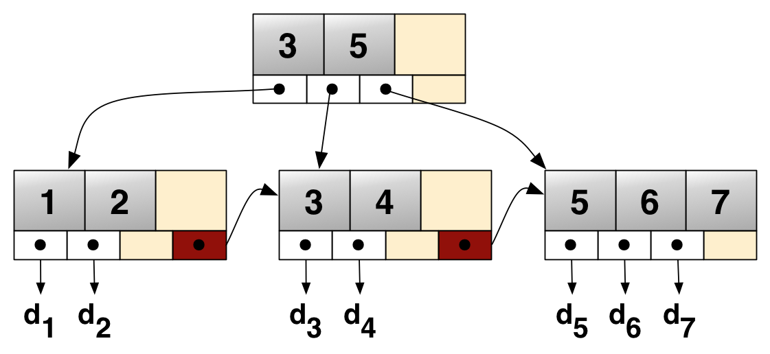
B+ tree construction — step-by-step worked exampleB+ tree construction — ধাপে ধাপে worked example
Problem: build a B+ tree of order \( n = 5 \) by inserting 12, 14, 19, 30, 21, 22, 13, 34, 18, 23, 38, 40 in this order. Order 5 means: a node has at most 5 pointers, so at most 4 keys.
Split rules (memorize): when a 5th key would enter a leaf, split it — the first \( \lceil 5/2 \rceil = 3 \) keys stay in the left leaf, the last 2 go to a new right leaf, and the FIRST key of the right leaf is copied up into the parent (copied, because in a B+ tree every key must also stay at the leaf level). If an internal node overflows, its middle key moves up instead (not needed in this problem).
Problem: order \( n = 5 \)-এর একটা B+ tree বানান, এই order-এ insert করে: 12, 14, 19, 30, 21, 22, 13, 34, 18, 23, 38, 40। Order 5 মানে: এক node-এ সর্বোচ্চ ৫টা pointer, তাই সর্বোচ্চ ৪টা key।
Split-এর নিয়ম (মুখস্থ রাখুন): leaf-এ ৫ নম্বর key ঢুকতে গেলে split করুন — প্রথম \( \lceil 5/2 \rceil = 3 \)টা key বাম leaf-এ থাকে, শেষ ২টা নতুন ডান leaf-এ যায়, আর ডান leaf-এর FIRST key parent-এ copy হয়ে উপরে যায় (copy, কারণ B+ tree-তে প্রতিটা key leaf level-এও থাকতেই হবে)। Internal node overflow করলে তার মাঝের key copy না হয়ে উপরে চলে যায় (এই problem-এ লাগবে না)।
| InsertInsert | What happensকী ঘটে | Tree afterপরের tree |
|---|---|---|
| 12, 14, 19, 30 | All fit in one leaf (4 keys = full but legal)সব এক leaf-এ ধরে (৪ key = full কিন্তু বৈধ) | [12 14 19 30] |
| 21 | SPLIT 1: sorted set {12,14,19,21,30} overflows → left [12 14 19], right [21 30], copy 21 up → new rootSPLIT 1: sorted {12,14,19,21,30} overflow → বাম [12 14 19], ডান [21 30], 21 copy হয়ে উপরে → নতুন root | [21] / [12 14 19] [21 30] |
| 22 | 22 ≥ 21 → right leaf, fits22 ≥ 21 → ডান leaf-এ, ধরে যায় | [21] / [12 14 19] [21 22 30] |
| 13 | 13 < 21 → left leaf, fits13 < 21 → বাম leaf-এ, ধরে যায় | [21] / [12 13 14 19] [21 22 30] |
| 34 | 34 ≥ 21 → right leaf, fits (now full)34 ≥ 21 → ডান leaf-এ, ধরে যায় (এখন full) | [21] / [12 13 14 19] [21 22 30 34] |
| 18 | SPLIT 2: {12,13,14,18,19} overflows → [12 13 14] and [18 19], copy 18 upSPLIT 2: {12,13,14,18,19} overflow → [12 13 14] আর [18 19], 18 copy হয়ে উপরে | [18 21] / [12 13 14] [18 19] [21 22 30 34] |
| 23 | SPLIT 3: {21,22,23,30,34} overflows → [21 22 23] and [30 34], copy 30 upSPLIT 3: {21,22,23,30,34} overflow → [21 22 23] আর [30 34], 30 copy হয়ে উপরে | [18 21 30] / [12 13 14] [18 19] [21 22 23] [30 34] |
| 38 | 38 ≥ 30 → last leaf, fits38 ≥ 30 → শেষ leaf-এ, ধরে যায় | [18 21 30] / [12 13 14] [18 19] [21 22 23] [30 34 38] |
| 40 | 40 ≥ 30 → last leaf, fits (4 keys = full but legal). DONE.40 ≥ 30 → শেষ leaf-এ, ধরে যায় (৪ key = full কিন্তু বৈধ)। শেষ। | [18 21 30] / [12 13 14] [18 19] [21 22 23] [30 34 38 40] |
Hash index (briefly)Hash index (সংক্ষেপে)
A hash index applies a hash function to the key: \( h(key) \) gives the bucket where the record sits. Equality search (WHERE sid = 101) is O(1) on average — even faster than a B+ tree. But hashing keeps NO order, so it is useless for range queries (BETWEEN, <, >) and sorting. Static hashing fixes the bucket count (overflow chains grow); extendible/dynamic hashing grows the directory as data grows.
Hash index key-এর উপর একটা hash function চালায়: \( h(key) \) বলে দেয় record কোন bucket-এ আছে। Equality search (WHERE sid = 101) গড়ে O(1) — B+ tree-র চেয়েও fast। কিন্তু hash-এ কোনো order থাকে না, তাই range query (BETWEEN, <, >) আর sorting-এ এটা অকেজো। Static hashing-এ bucket সংখ্যা fixed (overflow chain বাড়ে); extendible/dynamic hashing-এ data বাড়ার সাথে directory বাড়ে।
RAID Levels (Real Exam Topic!)RAID Levels (Real Exam Topic!)
Indexes make search fast, but the data itself lives on disks — and disks fail. RAID (Redundant Array of Independent Disks) combines several disks into one logical unit to get more speed, more safety (redundancy), or both. Each "level" is a different trade-off between performance, capacity, and how many disk failures you can survive.
Two building ideas: striping = split data into blocks and spread them across disks (many disks work in parallel → fast). Mirroring = keep a full copy of the data on another disk (a disk dies → the copy survives). Parity = store an extra XOR block; if one disk dies, its data can be rebuilt from the others plus the parity.
Index search fast করে, কিন্তু data নিজে থাকে disk-এ — আর disk fail করে। RAID (Redundant Array of Independent Disks) কয়েকটা disk-কে একটা logical unit বানায়, যাতে বেশি speed, বেশি safety (redundancy), বা দুটোই পাওয়া যায়। প্রতিটা "level" হলো performance, capacity আর কয়টা disk failure সহ্য করা যায় — এই তিনের আলাদা trade-off।
দুইটা মূল idea: striping = data-কে block-এ ভেঙে অনেক disk-এ ছড়িয়ে দেওয়া (অনেক disk একসাথে কাজ করে → fast)। Mirroring = data-র পুরো একটা copy আরেক disk-এ রাখা (একটা disk মরলে copy বেঁচে থাকে)। Parity = একটা বাড়তি XOR block রাখা; একটা disk মরলে বাকিগুলো আর parity থেকে তার data আবার বানানো যায়।
| LevelLevel | TechniqueTechnique | Min disksMin disk | Usable capacityUsable capacity | Failure toleranceFailure tolerance |
|---|---|---|---|---|
| RAID 0 | striping onlyশুধু striping | 2 | 100% (n) | 0 disks — 1 failure loses ALL data0টা disk — ১টা fail মানে সব data শেষ |
| RAID 1 | mirroringmirroring | 2 | 50% (n/2) | 1 disk (per mirror pair)১টা disk (প্রতি mirror pair-এ) |
| RAID 5 | striping + distributed paritystriping + distributed parity | 3 | (n−1)/n | exactly 1 diskঠিক ১টা disk |
| RAID 6 | striping + double paritystriping + double parity | 4 | (n−2)/n | any 2 disksযেকোনো ২টা disk |
| RAID 10 | mirror pairs, then stripemirror pair, তারপর stripe | 4 | 50% (n/2) | 1 per pair (up to n/2 if in different pairs)প্রতি pair-এ ১টা (আলাদা pair হলে n/2 পর্যন্ত) |
- RAID 0 (striping): blocks A1, A2, A3, A4 go round-robin across disks. Reads and writes are fast (parallel), and you use 100% of the space. But there is no redundancy: if any one disk fails, the whole array's data is gone. Use only for speed, never for important data.
- RAID 1 (mirroring): every block is written to two disks. Full redundancy — one disk of a pair can die and nothing is lost. Reads can be served by either disk (fast reads), but you only get 50% usable capacity.
- RAID 5 (striping + distributed parity): data is striped, and for each stripe one parity block (XOR of the data blocks) is stored — rotated across all disks so no single disk is the "parity disk". Needs at least 3 disks. Survives exactly 1 disk failure: the missing block is rebuilt as XOR of the surviving blocks. Usable capacity = (n−1)/n. Writes are a bit slower (parity must be updated).
- RAID 6: like RAID 5 but with two independent parity blocks per stripe — survives any 2 disk failures; capacity (n−2)/n; needs ≥ 4 disks.
- RAID 10 (1+0): make mirror pairs first, then stripe across the pairs — the speed of RAID 0 with the safety of RAID 1, at 50% capacity; needs ≥ 4 disks.
- RAID 0 (striping): block A1, A2, A3, A4 পালা করে disk-গুলোতে যায়। Read আর write fast (parallel), আর space-এর 100% ব্যবহার হয়। কিন্তু কোনো redundancy নেই: যেকোনো একটা disk fail করলেই পুরো array-র data শেষ। শুধু speed-এর জন্য, দরকারি data-র জন্য কখনো না।
- RAID 1 (mirroring): প্রতিটা block দুইটা disk-এ লেখা হয়। Full redundancy — pair-এর একটা disk মরলেও কিছু হারায় না। Read যেকোনো disk থেকে হতে পারে (fast read), কিন্তু usable capacity মাত্র 50%।
- RAID 5 (striping + distributed parity): data stripe হয়, আর প্রতি stripe-এর জন্য একটা parity block (data block-গুলোর XOR) রাখা হয় — সেটা ঘুরে ঘুরে সব disk-এ যায়, তাই আলাদা কোনো "parity disk" নেই। কমপক্ষে ৩টা disk লাগে। ঠিক ১টা disk failure সহ্য করে: হারানো block বেঁচে থাকা block-গুলোর XOR দিয়ে আবার বানানো যায়। Usable capacity = (n−1)/n। Write একটু slow (parity-ও update করতে হয়)।
- RAID 6: RAID 5-এর মতো, কিন্তু প্রতি stripe-এ দুইটা আলাদা parity block — যেকোনো ২টা disk failure সহ্য করে; capacity (n−2)/n; ≥ ৪টা disk লাগে।
- RAID 10 (1+0): আগে mirror pair বানায়, তারপর pair-গুলোর উপর stripe করে — RAID 0-এর speed আর RAID 1-এর safety একসাথে, 50% capacity-তে; ≥ ৪টা disk লাগে।
- RAID 0: everything is data → usable = 4 TB. Tolerates 0 failures.
- RAID 10: 2 mirror pairs, striped → usable = 4/2 = 2 TB. Tolerates 1 failure per pair.
- RAID 5: one disk's worth goes to parity → usable = (4−1) × 1 = 3 TB. Tolerates exactly 1 failure.
- RAID 0: সবটাই data → usable = 4 TB। ০টা failure সহ্য করে।
- RAID 10: ২টা mirror pair, তার উপর stripe → usable = 4/2 = 2 TB। প্রতি pair-এ ১টা failure সহ্য করে।
- RAID 5: এক disk-এর সমান জায়গা parity-তে যায় → usable = (4−1) × 1 = 3 TB। ঠিক ১টা failure সহ্য করে।
Practice Questions (Admission Style)Practice Questions (Admission Style)
Show Answerউত্তর দেখুন
Show Answerউত্তর দেখুন
Enroll(sid, cid, grade)) whose primary key is the pair. A foreign key on one side works only for 1:N.Enroll(sid, cid, grade)), যার primary key হলো জোড়াটা। এক পাশে foreign key শুধু 1:N-এর জন্য কাজ করে।Show Answerউত্তর দেখুন
COUNT(*) cannot appear inside WHERE, because WHERE filters rows BEFORE groups exist. Filtering on an aggregate must use HAVING, as option (d) correctly does.COUNT(*)-এর মতো aggregate function WHERE-এর ভিতরে বসতে পারে না, কারণ WHERE group তৈরি হওয়ার আগেই row filter করে। Aggregate দিয়ে filter করতে হলে HAVING লাগবে, যেমনটা (d)-তে ঠিকভাবে করা হয়েছে।Show Answerউত্তর দেখুন
SELECT S.name FROM Student S
LEFT JOIN Enroll E ON S.sid = E.sid;SELECT S.name FROM Student S
LEFT JOIN Enroll E ON S.sid = E.sid;Show Answerউত্তর দেখুন
Show Answerউত্তর দেখুন
SELECT DISTINCT. \( \sigma \) picks rows, not columns.SELECT DISTINCT-এর মতো। \( \sigma \) row বাছে, column না।Show Answerউত্তর দেখুন
Show Answerউত্তর দেখুন
Show Answerউত্তর দেখুন
-- (i) join all three tables
SELECT DISTINCT S.name
FROM Student S
JOIN Enroll E ON S.sid = E.sid
JOIN Course C ON E.cid = C.cid
WHERE C.title = 'Database';

-- (ii) aggregate + group filter
SELECT dept, COUNT(*) AS total
FROM Student
GROUP BY dept
HAVING COUNT(*) >= 2;
Reasoning: (i) needs a path Student → Enroll → Course to reach the title, joined on sid and cid. (ii) counts per group, and the "at least 2" condition is on the aggregate, so it must go in HAVING, not WHERE. With our sample data, (i) returns Rahim, Karim and (ii) returns (CSE, 2).
-- (i) তিনটা table join
SELECT DISTINCT S.name
FROM Student S
JOIN Enroll E ON S.sid = E.sid
JOIN Course C ON E.cid = C.cid
WHERE C.title = 'Database';

-- (ii) aggregate + group filter
SELECT dept, COUNT(*) AS total
FROM Student
GROUP BY dept
HAVING COUNT(*) >= 2;
ব্যাখ্যা: (i)-এ title পেতে Student → Enroll → Course path লাগবে, sid আর cid দিয়ে join। (ii)-এ group ধরে গোনা হয়, আর "কমপক্ষে ২" condition-টা aggregate-এর উপর, তাই সেটা WHERE-এ না, HAVING-এ যাবে। আমাদের sample data-তে (i) দেয় Rahim, Karim আর (ii) দেয় (CSE, 2)।
Show Answerউত্তর দেখুন
(i) \( \pi_{name}(Student \bowtie \sigma_{cid='C1'}(Enroll)) \)
First filter Enroll to only C1 rows (σ), then natural join with Student on sid to attach names, then project name (π). Filtering before joining is also the efficient order.
(ii) \( \pi_{sid}(Student) - \pi_{sid}(Enroll) \)
All student ids minus the ids that appear in Enroll leaves exactly the students who never enrolled. Set difference (−) is the natural tool for "NO / not any" questions.
(i) \( \pi_{name}(Student \bowtie \sigma_{cid='C1'}(Enroll)) \)
আগে Enroll থেকে শুধু C1-এর row filter করুন (σ), তারপর sid দিয়ে Student-এর সাথে natural join করে name আনুন, শেষে name project করুন (π)। Join-এর আগে filter করাটাই efficient order।
(ii) \( \pi_{sid}(Student) - \pi_{sid}(Enroll) \)
সব student-এর id থেকে Enroll-এ থাকা id বাদ দিলে ঠিক তারাই থাকে যারা কখনো enroll করেনি। "কোনোটাই না / NO" ধরনের প্রশ্নে set difference (−)-ই আসল হাতিয়ার।
Show Answerউত্তর দেখুন
\( (AB)^+ \): start {A,B} → AB→C adds C → C→D adds D → {A,B,C,D}. So AB is a key.
B never appears on any right side, so B is in EVERY candidate key. Test B alone: \( B^+ = \{B\} \) — not a key. Test pairs containing B:
- \( (AB)^+ = ABCD \) ✓
- \( (CB)^+ \): {B,C} → C→D adds D → D→A adds A → ABCD ✓
- \( (DB)^+ \): {B,D} → D→A adds A → AB→C adds C → ABCD ✓
Candidate keys: AB, BC, BD. All are minimal (B alone fails, and A, C, D alone add nothing without B).
\( (AB)^+ \): শুরু {A,B} → AB→C থেকে C → C→D থেকে D → {A,B,C,D}। তাই AB একটা key।
B কোনো FD-র ডান পাশে নেই, তাই B প্রতিটা candidate key-তে থাকবে। শুধু B দেখুন: \( B^+ = \{B\} \) — key না। এবার B-সহ জোড়াগুলো:
- \( (AB)^+ = ABCD \) ✓
- \( (CB)^+ \): {B,C} → C→D থেকে D → D→A থেকে A → ABCD ✓
- \( (DB)^+ \): {B,D} → D→A থেকে A → AB→C থেকে C → ABCD ✓
Candidate key: AB, BC, BD। সবগুলোই minimal (শুধু B fail করে, আর B ছাড়া শুধু A, C বা D কিছুই দেয় না)।
Show Answerউত্তর দেখুন
2NF step (remove partial dependencies): customer_id and customer_name depend on order_id alone; product_name depends on product_id alone — both are parts of the key. Split:
- OrderInfo(order_id, customer_id, customer_name)
- Product(product_id, product_name)
- OrderLine(order_id, product_id, qty) — qty depends on the full key, so it stays.
3NF step (remove transitive dependency): in OrderInfo, order_id → customer_id → customer_name is non-key → non-key. Split again:
- Orders(order_id, customer_id)
- Customer(customer_id, customer_name)
Final 3NF schema: Orders(order_id, customer_id), Customer(customer_id, customer_name), Product(product_id, product_name), OrderLine(order_id, product_id, qty). Every FD now has a key on its left side, so this is even BCNF.
2NF step (partial dependency দূর): customer_id আর customer_name শুধু order_id-এর উপর নির্ভর করে; product_name শুধু product_id-এর উপর — দুটোই key-এর অংশ। ভাঙুন:
- OrderInfo(order_id, customer_id, customer_name)
- Product(product_id, product_name)
- OrderLine(order_id, product_id, qty) — qty পুরো key-এর উপর নির্ভর করে, তাই এখানেই থাকবে।
3NF step (transitive dependency দূর): OrderInfo-তে order_id → customer_id → customer_name হলো non-key → non-key। আবার ভাঙুন:
- Orders(order_id, customer_id)
- Customer(customer_id, customer_name)
Final 3NF schema: Orders(order_id, customer_id), Customer(customer_id, customer_name), Product(product_id, product_name), OrderLine(order_id, product_id, qty)। এখন প্রতিটা FD-র বাম পাশে key আছে, তাই এটা BCNF-ও বটে।
Show Answerউত্তর দেখুন
(i) A appears on no right side → A is in every key. \( A^+ = \{A\} \), so A alone fails. \( (AB)^+ = \{A,B,C\} \) ✓ and \( (AC)^+ \): C→B adds B → \{A,B,C\} ✓. Candidate keys: AB and AC. So every attribute is prime.
(ii) 3NF: yes. The FD C → B has a non-superkey left side, but B is a prime attribute, and 3NF allows key → anything OR anything → prime. BCNF: no. C → B with C not a superkey directly violates BCNF.
(iii) If we decompose for BCNF into (C, B) and (A, C), the FD AB → C can no longer be checked inside a single table — the decomposition is lossless but NOT dependency preserving. This is the standard example showing why "BCNF always" is not free, and why 3NF is sometimes accepted instead.
(i) A কোনো FD-র ডান পাশে নেই → A প্রতিটা key-তে থাকবে। \( A^+ = \{A\} \), তাই শুধু A fail। \( (AB)^+ = \{A,B,C\} \) ✓ আর \( (AC)^+ \): C→B থেকে B → \{A,B,C\} ✓। Candidate key: AB আর AC। তাই প্রতিটা attribute-ই prime।
(ii) 3NF: হ্যাঁ। C → B FD-র বাম পাশ superkey না, কিন্তু B একটা prime attribute — 3NF allow করে: key → যেকোনো কিছু অথবা যেকোনো কিছু → prime। BCNF: না। C superkey না হয়েও C → B আছে — এটা সরাসরি BCNF ভাঙে।
(iii) BCNF-এর জন্য (C, B) আর (A, C)-তে ভাঙলে AB → C FD-টা আর কোনো এক table-এর ভিতরে check করা যায় না — decomposition-টা lossless কিন্তু dependency preserving না। এটাই standard example যা দেখায় "সবসময় BCNF" free না, আর কখনো কখনো 3NF-ই মেনে নেওয়া হয়।
Show Answerউত্তর দেখুন
List the conflict pairs (same item, different transactions, at least one write):
- On A: R1(A) before W2(A) → edge T1 → T2. (R2–W2 are the same transaction — no edge.)
- On B: R3(B) before W1(B) → edge T3 → T1; W1(B) before R2(B) → edge T1 → T2.
Graph edges: T3 → T1, T1 → T2. No cycle → conflict serializable. Topological order: T3, T1, T2 — the schedule behaves exactly like running T3 fully, then T1, then T2.
Conflict pair-গুলো বের করুন (একই item, আলাদা transaction, অন্তত একটা write):
- A-তে: R1(A) আগে, W2(A) পরে → edge T1 → T2। (R2–W2 একই transaction-এর — edge হয় না।)
- B-তে: R3(B) আগে, W1(B) পরে → edge T3 → T1; W1(B) আগে, R2(B) পরে → edge T1 → T2।
Graph-এর edge: T3 → T1, T1 → T2। কোনো cycle নেই → conflict serializable। Topological order: T3, T1, T2 — schedule-টা ঠিক T3 পুরো, তারপর T1, তারপর T2 চালানোর মতো আচরণ করে।
Show Answerউত্তর দেখুন
(i) Each internal node fans out to at most 4 children. With 3 levels of internal nodes: \( 4 \times 4 \times 4 = 64 \) leaf pointers. In general, height \( h \) with fan-out \( f \) reaches \( f^h \) leaves — growth is exponential in height.
(ii) A binary search tree has fan-out 2, so 1 million records need height about \( \log_2 10^6 \approx 20 \) — about 20 disk reads per search. A real B+ tree node fills a whole disk block (fan-out 100+), so height is about \( \log_{100} 10^6 = 3 \) — about 3 disk reads. Since disk reads dominate cost, fewer levels = much faster. Plus, linked leaves give cheap range scans, which a plain BST does not.
(i) প্রতিটা internal node সর্বোচ্চ ৪টা child-এ যায়। ৩ level internal node হলে: \( 4 \times 4 \times 4 = 64 \)টা leaf pointer। সাধারণভাবে, fan-out \( f \) আর height \( h \) হলে \( f^h \)টা leaf — height-এর সাথে exponential বৃদ্ধি।
(ii) Binary search tree-র fan-out 2, তাই ১০ লাখ record-এ height প্রায় \( \log_2 10^6 \approx 20 \) — প্রতি search-এ প্রায় ২০টা disk read। আসল B+ tree-র এক node পুরো একটা disk block ভরে (fan-out ১০০+), তাই height প্রায় \( \log_{100} 10^6 = 3 \) — মাত্র ৩টা disk read। খরচের বড় অংশই disk read, তাই কম level মানে অনেক faster। তার উপর linked leaf-এ range scan সস্তা, যা সাধারণ BST-তে নেই।
Employee(emp_id, name, salary). Write a trigger that records every salary change into SalaryLog(emp_id, old_salary, new_salary, changed_on). (iii) Give one case where using a trigger is a bad idea.Employee(emp_id, name, salary)। এমন একটা trigger লিখুন যা প্রতিটা salary change SalaryLog(emp_id, old_salary, new_salary, changed_on)-এ record করে। (iii) কোন একটা case বলুন যেখানে trigger ব্যবহার করা খারাপ idea।Show Answerউত্তর দেখুন
(i) A trigger is a stored program attached to a table that the database fires automatically when an INSERT, UPDATE, or DELETE happens — nobody calls it by hand. BEFORE triggers run before the change is applied (good for validating or fixing values); AFTER triggers run after it (good for logging). A row-level trigger (FOR EACH ROW) fires once per changed row and can read OLD and NEW values; a statement-level trigger fires once per statement, however many rows changed.
-- (ii)
CREATE TRIGGER salary_audit
AFTER UPDATE ON Employee
FOR EACH ROW
WHEN (NEW.salary <> OLD.salary)
BEGIN
  INSERT INTO SalaryLog(emp_id, old_salary, new_salary, changed_on)
  VALUES (OLD.emp_id, OLD.salary, NEW.salary, CURRENT_DATE);
END;
Why each choice: AFTER — we log only changes that really happened; FOR EACH ROW — each employee gets their own log row; the WHEN guard skips updates that did not touch the salary; OLD/NEW give the values before and after.
(iii) Bad idea: putting heavy business logic in triggers. They run invisibly, so bugs are hard to trace; a trigger can fire another trigger and create chains or loops; and a row-level trigger on a bulk UPDATE of a million rows fires a million times.
(i) Trigger হলো table-এর সাথে লাগানো একটা stored program, যা INSERT, UPDATE বা DELETE ঘটলে database নিজে থেকেই fire করে — কেউ হাতে call করে না। BEFORE trigger change apply হওয়ার আগে চলে (value validate বা ঠিক করার জন্য ভালো); AFTER trigger পরে চলে (log-এর জন্য ভালো)। Row-level trigger (FOR EACH ROW) প্রতিটা বদলানো row-এর জন্য একবার fire হয়, আর OLD/NEW value পড়তে পারে; statement-level trigger প্রতি statement-এ একবারই fire হয়, যত row-ই বদলাক।
-- (ii)
CREATE TRIGGER salary_audit
AFTER UPDATE ON Employee
FOR EACH ROW
WHEN (NEW.salary <> OLD.salary)
BEGIN
  INSERT INTO SalaryLog(emp_id, old_salary, new_salary, changed_on)
  VALUES (OLD.emp_id, OLD.salary, NEW.salary, CURRENT_DATE);
END;
প্রতিটা choice-এর কারণ: AFTER — শুধু সত্যিই ঘটে যাওয়া change log হয়; FOR EACH ROW — প্রতিটা employee-র নিজের log row হয়; WHEN guard সেই update বাদ দেয় যেখানে salary বদলায়নি; OLD/NEW দেয় আগের আর পরের value।
(iii) খারাপ idea: ভারী business logic trigger-এ রাখা। এগুলো অদৃশ্যভাবে চলে, তাই bug খুঁজে বের করা কঠিন; এক trigger আরেকটা fire করে chain বা loop বানাতে পারে; আর ১০ লাখ row-এর bulk UPDATE-এ row-level trigger ১০ লাখ বার fire হয়।
Show Answerউত্তর দেখুন
Insert 10, 20, 5: one leaf, sorted: [5 10 20] (3 keys = full but legal).
Insert 15 — SPLIT 1: {5, 10, 15, 20} overflows. Left keeps [5 10], right gets [15 20], copy 15 up as a new root.
        [15]
       /    \
 [5 10] -> [15 20]
Insert 25: 25 ≥ 15 → right leaf: [15 20 25].
Insert 30 — SPLIT 2: {15, 20, 25, 30} overflows. Left keeps [15 20], right gets [25 30], copy 25 into the root.
        [15 | 25]
       /    |     \
 [5 10] -> [15 20] -> [25 30]
Insert 8: 8 < 15 → first leaf: [5 8 10]. Final tree:
        [15 | 25]
       /    |     \
 [5 8 10] -> [15 20] -> [25 30]
Checks: all 7 keys are in the leaves (3 + 2 + 2 = 7), leaves are sorted and linked, the copied-up keys 15 and 25 still appear in leaves, and every leaf has at least \( \lceil 3/2 \rceil = 2 \) keys.
Insert 10, 20, 5: একটা leaf, sorted: [5 10 20] (৩ key = full কিন্তু বৈধ)।
Insert 15 — SPLIT 1: {5, 10, 15, 20} overflow করে। বাম রাখে [5 10], ডান পায় [15 20], 15 copy হয়ে নতুন root হয়।
        [15]
       /    \
 [5 10] -> [15 20]
Insert 25: 25 ≥ 15 → ডান leaf: [15 20 25]।
Insert 30 — SPLIT 2: {15, 20, 25, 30} overflow করে। বাম রাখে [15 20], ডান পায় [25 30], 25 copy হয়ে root-এ যায়।
        [15 | 25]
       /    |     \
 [5 10] -> [15 20] -> [25 30]
Insert 8: 8 < 15 → প্রথম leaf: [5 8 10]। Final tree:
        [15 | 25]
       /    |     \
 [5 8 10] -> [15 20] -> [25 30]
Check: ৭টা key-ই leaf-এ আছে (3 + 2 + 2 = 7), leaf-গুলো sorted আর linked, উপরে copy হওয়া 15 আর 25 leaf-এও আছে, আর প্রতিটা leaf-এ কমপক্ষে \( \lceil 3/2 \rceil = 2 \)টা key আছে।
Show Answerউত্তর দেখুন
Raw total = 6 × 2 = 12 TB.
(i) Usable capacity:
- RAID 0: n·d = 6 × 2 = 12 TB (all data, no redundancy).
- RAID 10: (n/2)·d = 3 × 2 = 6 TB (3 mirror pairs).
- RAID 5: (n−1)·d = 5 × 2 = 10 TB (one disk's worth of parity).
- RAID 6: (n−2)·d = 4 × 2 = 8 TB (two disks' worth of parity).
(ii) Failure tolerance: RAID 0 = 0 (one failure destroys everything). RAID 10 = 1 per mirror pair (best case 3, but two failures in the SAME pair lose data — so guaranteed only 1). RAID 5 = exactly 1. RAID 6 = any 2.
(iii) Pick RAID 5. It survives the required 1 disk failure and gives 10 TB usable — more than RAID 10 (6 TB) and RAID 6 (8 TB). The trade-off is slower writes (parity update) and a risky rebuild window, but the question only demands 1-failure tolerance with maximum space, and RAID 5 wins that exactly.
Raw মোট = 6 × 2 = 12 TB।
(i) Usable capacity:
- RAID 0: n·d = 6 × 2 = 12 TB (সবই data, কোনো redundancy নেই)।
- RAID 10: (n/2)·d = 3 × 2 = 6 TB (৩টা mirror pair)।
- RAID 5: (n−1)·d = 5 × 2 = 10 TB (এক disk-এর সমান parity)।
- RAID 6: (n−2)·d = 4 × 2 = 8 TB (দুই disk-এর সমান parity)।
(ii) Failure tolerance: RAID 0 = 0 (১টা failure-এই সব শেষ)। RAID 10 = প্রতি mirror pair-এ ১টা (best case ৩টা, কিন্তু একই pair-এ ২টা failure হলে data হারায় — তাই guarantee শুধু ১টা)। RAID 5 = ঠিক ১টা। RAID 6 = যেকোনো ২টা।
(iii) RAID 5 নিন। এটা দরকারি ১টা disk failure সহ্য করে আর 10 TB usable দেয় — RAID 10 (6 TB) আর RAID 6 (8 TB)-এর চেয়ে বেশি। Trade-off হলো write একটু slow (parity update) আর rebuild-এর সময়টা risky, কিন্তু প্রশ্ন চেয়েছে শুধু ১-failure tolerance আর সর্বোচ্চ space — সেটা RAID 5-ই ঠিকঠাক দেয়।
Show Answerউত্তর দেখুন
(i) Both transactions read A = 100. T1 writes 100 + 50 = 150. Then T2 writes 100 − 30 = 70 — computed from the stale 100, so it overwrites T1's 150. Final A = 70, but the correct value is 100 + 50 − 30 = 120.
(ii) This is the lost update anomaly: T1's write is overwritten and lost because T2 read the old value before T1 wrote.
(iii) With strict 2PL, each transaction takes an X lock on A before touching it and holds it until commit:
- T1: X-lock(A) granted → R1(A) = 100.
- T2: requests X-lock(A) → BLOCKED (T1 holds it). T2 waits.
- T1: A = 150, W1(A), commit → lock released.
- T2: X-lock(A) granted → R2(A) = 150 (fresh value!), A = 150 − 30 = 120, W2(A), commit.
Final A = 120 — correct. The schedule is now equivalent to serial T1 → T2, so no update is lost.
(i) দুই transaction-ই A = 100 পড়ে। T1 লেখে 100 + 50 = 150। তারপর T2 লেখে 100 − 30 = 70 — পুরনো 100 থেকে হিসাব করা, তাই এটা T1-এর 150-কে overwrite করে। Final A = 70, কিন্তু সঠিক value 100 + 50 − 30 = 120।
(ii) এটা lost update anomaly: T1-এর write overwrite হয়ে হারিয়ে যায়, কারণ T1 লেখার আগেই T2 পুরনো value পড়ে ফেলেছিল।
(iii) Strict 2PL-এ প্রতিটা transaction A-তে হাত দেওয়ার আগে X lock নেয় আর commit পর্যন্ত ধরে রাখে:
- T1: X-lock(A) পায় → R1(A) = 100।
- T2: X-lock(A) চায় → BLOCKED (T1 ধরে আছে)। T2 অপেক্ষা করে।
- T1: A = 150, W1(A), commit → lock ছাড়ে।
- T2: X-lock(A) পায় → R2(A) = 150 (fresh value!), A = 150 − 30 = 120, W2(A), commit।
Final A = 120 — সঠিক। Schedule-টা এখন serial T1 → T2-এর সমান, তাই কোনো update হারায় না।